Intro to Statistics: Part 19: Confidence Intervals
Continuing with the Norwegian heights example... suppose you were tasked with figuring out the mean average height of the Norwegian population. The only way to determine the true population mean is to measure every single member of the population. That's impractical however, so instead you sample the heights of 30 Norwegians and calculate the sample mean, which gives you an estimate of the true population mean.
How confident are you in your estimate?
Confidence in the estimate of an unknown population parameter is typically expressed using a confidence interval. A confidence interval is a range of values that you believe, with a certain degree of confidence, contains the true value of the unknown parameter.
The concept of confidence intervals is best illustrated with an example. Let's pretend that your Norwegian sample mean is 68.9in, and the sample standard deviation is 3in. Given this information we can construct a sampling distribution of the mean, using the sample mean and sample standard deviation as estimates of the true population mean and true population standard deviation.
N <- 30
sample.mean <- 68.9
sample.sd <- 3

sampling.se <- sample.sd / sqrt(N)  # standard error of the mean

x <- seq(66,72,0.01)
ggplot() +
    stat_function(aes(x=x),
                  fun=dnorm,
                  arg=list(mean=sample.mean, sd=sampling.se),
                  size=1,
                  colour="blue") +
    ggtitle("Sampling distribution of the mean\n(sample size N=30)") +
    geom_hline(y=0, colour="darkgray") +
    geom_vline(x=sample.mean, linetype="dashed", colour="blue", size=1) +
    ylab("Probability density") +
    xlab("Sample means")  +
    scale_x_continuous(breaks=66:72, labels=66:72)

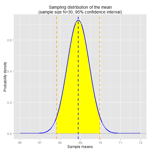
Confidence intervals are expressed with a certain degree of confidence, for example a 90% confidence interval, 95% confidence interval, 99% confidence interval, etc. The degree of confidence corresponds to the probability of finding the sample mean within a certain range. We can determine the range using the sampling distribution. The sampling distribution gives us the probabilities of observing various sample means for a given sample size, in this case for sample size N=30.
For a 95% confidence interval, we're looking for the range of sample means that constitute 95% of the sampling distribution, centered around our estimate of the true population mean, which we've estimated using the sample mean. We know that our sample mean sits at the center of the sampling distribution, so we know that 50% of sample means lie below the estimate and 50% lie above the estimate. If we want the 95% confidence interval, then we're looking at the range from 47.5% below and 47.5% above the sample mean. In terms of quantiles, this is the 2.5% quantile and 97.5% quantile, respectively. We can determine these values using the qnorm function.
conf.int.95.lower.bound <- qnorm(0.025, mean=sample.mean, sd=sampling.se)
## 67.82648

conf.int.95.upper.bound <- qnorm(0.975, mean=sample.mean, sd=sampling.se)
## 69.97352
This gives us our 95% confidence interval: 67.83in thru 69.97in. Note that our sample mean lies directly in the center of that interval.
How about a 90% confidence interval? In that case, we're looking at the range from 45% below and 45% above the sample mean, which corresponds to quantiles 5% and 95%:
conf.int.90.lower.bound <- qnorm(0.05, mean=sample.mean, sd=sampling.se)
## 67.99908

conf.int.90.upper.bound <- qnorm(0.95, mean=sample.mean, sd=sampling.se)
## 69.80092
This gives us a 90% confidence interval of 68.00in thru 69.80in. Again, the sample mean lies directly in the center of the interval.
Note that the 90% confidence interval is smaller than the 95% interval. This is because we're less confident in this range (90% confidence vs 95% confidence), because the range is smaller.
The charts below show the 90% and 95% confidence intervals:

Misinterpreting the confidence interval
One thing to note about confidence intervals. They're often misinterpreted as the probability that the true population parameter lies within the interval. In the context of this example, that would be like saying there's a 90% probability that the true population mean lies within the range 68.0in to 69.8in. This is a misinterpretation.
The confidence interval merely states how confident you are in the estimated range. The degree of confidence has more to do with the procedure you used and the parameters of your experiment (e.g. sample size), rather than anything having to do with the true population parameter.
Think of it this way. The confidence interval is calculated from the sampling distribution, which depends in part on the sample size. Imagine if we increased the sample size. The sampling distribution would change, which would affect the confidence interval. Then we'd have two separate 95% confidence intervals: the one for the smaller sample size, and the one for the larger sample size.
How can two different intervals both have the same 95% probability of including the true population mean? They can't! Because that's not what the confidence interval tells us! The true population mean either does or does not lie in the interval. The confidence interval merely expresses our confidence -- not a probability -- that the interval indeed contains the true population mean.
Computing confidence intervals using the t-distribution
If your sample size is small (N < 30 is usually the rule of thumb), then you should use a t-distribution to estimate the sampling distribution of the mean, not a normal distribution as we did above. Recall that the t-distribution is a family of curves, each curve identified by the degrees of freedom. Our sample size is N=30, so the degrees of freedom is N-1=29.
We can use the qt function to determine the 0.025 and 0.975 quantile t-scores, just as we did above using the qnorm function:
conf.int.95.lower.bound.tscore <- qt(0.025, df=N-1)
## -2.04523

conf.int.95.upper.bound.tscore <- qt(0.975, df=N-1)
## 2.04523
The chart below plots the 95% confidence interval on the t-distribution curve for degrees of freedom = 29.

The orange lines are the lower and upper bound t-scores for the 95% confidence interval. To convert the t-score back to the original units of inches, we need to "de-normalize" it by multiplying by the standard deviation of the sampling distribution (a.k.a. the standard error of the mean) and adding back in the sample mean:

conf.int.95.lower.bound.tscore * sampling.se + sample.mean
## 67.77978

conf.int.95.upper.bound.tscore * sampling.se + sample.mean
## 70.02022
This gives us a 95% confidence interval of 67.78in thru 70.02in, which is slightly larger than the 95% confidence interval derived above from the normal distribution: 67.83in thru 69.97in. This makes sense, since the t-distribution has "thicker tails" than the normal distribution, in order to account for greater variability due to the small sample size. The difference is meager in this case, since our sample size is big enough such that the t-distribution curve closely approximates a normal distribution.
Recap
- A random variable is described by the characteristics of its distribution
- The expected value, E[X], of a distribution is the weighted average of all outcomes. It's the center of mass of the distribution.
- The variance, Var(X), is the "measure of spread" of a distribution.
- The standard deviation of a distribution is the square root of its variance
- A probability density function for continuous random variables takes an outcome value as input and returns the probability density for the given outcome
- The probability of observing an outcome within a given range can be determined by computing the area under the curve of the probability density function within the given range.
- A probability mass function for discrete random variables takes an outcome value as input and returns the actual probability for the given outcome
- A sample is a subset of a population. Statistical methods and principles are applied to the sample's distribution in order to make inferences about the true distribution -- i.e. the distribution across the population as a whole
- The sample variance is a biased estimate of the true population variance. The bias can be adjusted for by dividing the sum-of-squares by n-1 instead of n, where n is the sample size.
- A summary statistic is a value that summarizes sample data, e.g. the mean or the variance
- A sampling distribution is the distribution of a summary statistic (e.g. the mean) calculated from multiple samples drawn from an underlying random variable distribution
- The Central Limit Theorem states that, regardless of the underlying distribution, the sampling distribution of the mean is normally distributed, with its mean equal to the underlying population mean and its variance equal to the underlying population variance divided by the sample size
- An outcome's z-score is calculated by taking the difference between the outcome and the mean, then dividing by the standard deviation. A z-score is in units of standard deviations.
- A statistical significance test gives the probability of observing a given outcome under the assumption of a null hypothesis. The probability is known as the p-value for the test. A p-value <= 0.05 is typically considered significant.
- A Type I error, a.k.a. a "false positive", is when you incorrectly detect an effect in the sample data even though no real effect exists
- A Type II error, a.k.a. a "false negative", is when you incorrectly fail to detect an effect in the sample data even though a real effect truly exists
- The significance level, α, for a statistical significance test is the maximum allowed p-value that is considered significant. This is also known as the Type I error rate
- The Type II error rate, β, is the probability of incurring a Type II error (false negative)
- The t-distribution is used for statistical significance tests when the sample size is small and/or when the true population variance is unknown and therefore estimated from the sample.
- The sampling distribution of the variance follows a scaled chi-squared distribution with degrees of freedom equal to n-1, where n is the sample size.
- Analysis of variance and F-tests are used for statistical significance testing between three or more samples.