Intro to Statistics: Part 17: F-test (ANOVA) Significance Testing Between Three or more Samples
In the previous article we saw how t-tests are used for conducting a significance test between two samples. In this article we will look at how to use F-tests to conduct a signficance test between three or more samples.
F-tests are included in a set of statistical methods known as analysis of variance, or ANOVA for short. ANOVA methods analyze the variance of datasets composed of multiple groups (or samples) of data in order to investigate statistical relationships between groups, within groups, and in the interaction of groups.
F-tests analyze the variance across multiple samples (groups) by breaking down the variance into components:
- The overall variance of the entire dataset across all samples
- The variance within each sample
- The variance between samples
The idea is to compare the variance between samples to the variance within samples. The null hypothesis for the significance test typically assumes that the variance between samples should be no different than the variance within samples. If, however, the variance between samples is large compared to the variance within samples, then we might conclude that the difference between samples is significant.
The F-score
Analagous to t-scores, F-tests generate an F-score, which is then plotted on an F-distribution in order to determine the p-value of the significance test. The F-score is informally defined as:

If the variance between samples is rougly the same as the variance within samples, then the F-score will be about 1. An F-score of 1 is equivalent to a t-score of 0. It's basically saying that there's no measurable difference between the samples, so the null hypothesis (which assumes no difference) is accepted and the alternative hypothesis (that there's a statistically significant difference between samples) is rejected.
The variance between samples is defined as:

Note that this is the same as your basic definition of sample variance -- i.e. sum-of-squares divided by degrees of freedom. Similarly, variance within samples is calculated by:

For the moment let's set aside the degrees of freedom and just focus on how to compute the sum-of-squares. The sum-of-squares within samples is straightforward: just sum the squared diffs for each sample, as you normally would if you were computing sample variance.

The sum-of-squares between samples is a little less straightforward. For each sample, you compute the squared difference between the sample mean and the overall mean, where the overall mean is the mean across all samples. The squared diff is then multiplied by the sample size, so that each sample's squared diff is weighted by the number of observations in that sample.

It can be shown algebraically that the sum-of-squares within samples and the sum-of-squares between samples add up to the total overall sum-of-squares across all samples.

Now let's turn to the degrees of freedom. The degrees of freedom within samples is simply the sum of the degrees of freedom for each sample.
The degrees of freedom between samples is equal to the number of samples minus 1. Recall that the degrees of freedom is equal to the number of ways the statistic can vary, which in this case is equal to the number of sample means, minus 1 for the use of the intermediate variable, the overall mean.

Note that the degrees of freedom for each sample is the sample size minus 1, so the degrees of freedom within samples is the total number of observations across all samples, minus 1 for each sample. Putting it all together, the equation for F-score can be written as:
Example
Let's do an example. We need some sample data, so let's create our own. Let's pretend we're investigating the differences in height between various sports players, say basketball players, football players, and horse jockeys (or something... the context doesn't really matter). We'll use rnorm to generate random sample data. rnorm takes a mean and standard deviation as parameters, which define the normal distribution from which rnorm generates random values. We'll use different means and standard deviations for the three samples. This way we know for a fact there's a real difference between the three samples. The sample size for all three samples is the same, n1 = n2 = n3 = 30.
set.seed(1)
n1 <- 30
n2 <- 30
n3 <- 30
s1 <- rnorm( n1, mean=67, sd=3 )
s2 <- rnorm( n2, mean=68.5, sd=2.5)
s3 <- rnorm( n3, mean=72, sd=4 )
First let's compute the sum-of-squares within samples:
s1.ss <- sum( (s1 - mean(s1))^2 )
s2.ss <- sum( (s2 - mean(s2))^2 )
s3.ss <- sum( (s3 - mean(s3))^2 )
ss.within = s1.ss + s2.ss + s3.ss
Next up is the sum-of-squares between samples:
s.overall <- c(s1, s2, s3)
s1.between <- ( mean(s1) - mean(s.overall) )^2 * n1
s2.between <- ( mean(s2) - mean(s.overall) )^2 * n2
s3.between <- ( mean(s3) - mean(s.overall) )^2 * n3
ss.between <- s1.between + s2.between + s3.between
Note that the total overall sum-of-squares across all samples is equal to the sum of the sum-of-squares between and within samples.
s.overall.ss <- sum( (s.overall - mean(s.overall))^2 )
## 1190.591

ss.within + ss.between
## 1190.591
Next we compute the degrees of freedom both between and within samples and the f-score:
I <- 3      # Number of samples
df.within <- n1 + n2 + n3 - I
df.between <- I - 1

f <- ( ss.between / df.between ) / (ss.within / df.within)
## 24.15851
To determine the corresponding p-value, we can use the pf function. Similar to the pnorm and pt functions, the pf function returns probabilites associated with the F-distribution. The F-distribution is a family of distribution curves, where each curve is distinguished by the two degrees of freedom used in the F-score calculation. The two degrees of freedom are passed as parameters to the pf function. The degrees of freedom between samples goes first.
p.value <- 1 - pf(f, df.between, df.within)
## 4.521223e-09
That's an extraordinarily small probability. It represents the probability that the difference we observe between samples is due to random chance (the null hypothesis), as opposed to being due to some real difference between the samples (the alternative hypothesis). In this case we'd reject the null hypothesis and go with the alternative. This is the result we expected, given that we created the sample data ourselves and know for a fact there are real differences between the samples.
The aov function in R
R provides a function called aov that conducts the analysis of variance for us and gives us the resulting F-score and p-value. In order to use it, we have to put all the sample data in a single vector and use a factor variable to identify the different samples:
s.factor <- factor( c( rep(1,n1), rep(2,n2), rep(3,n3) ) )
summary( aov(s.overall ~ s.factor))
##             Df Sum Sq Mean Sq F value   Pr(>F)
## s.factor     2  425.1   212.6   24.16 4.52e-09
Note that the F-score (F value) and p-value (Pr(>F)) are the same as the values we calculated manually above.
Charting the F-distribution
To finish off the example, let's chart the probability density of the F-distribution curve that corresponds to the degrees of freedom in our example.
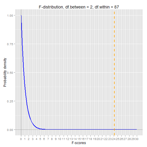
The vertical orange line is our F-score. As you can see it's way out along the tail of the distribution, which explains the extremely low p-value. The p-value represents the probability of seeing an F-score as extreme as (greater than) the one we got.
The chart below shows several curves in the F-distribution family. F-distribution curves resemble chi-squared distribution curves, which makes sense since both are based on the distribution of variances.

Source: wikipedia
Recap
- A random variable is described by the characteristics of its distribution
- The expected value, E[X], of a distribution is the weighted average of all outcomes. It's the center of mass of the distribution.
- The variance, Var(X), is the "measure of spread" of a distribution.
- The standard deviation of a distribution is the square root of its variance
- A probability density function for continuous random variables takes an outcome value as input and returns the probability density for the given outcome
- The probability of observing an outcome within a given range can be determined by computing the area under the curve of the probability density function within the given range.
- A probability mass function for discrete random variables takes an outcome value as input and returns the actual probability for the given outcome
- A sample is a subset of a population. Statistical methods and principles are applied to the sample's distribution in order to make inferences about the true distribution -- i.e. the distribution across the population as a whole
- The sample variance is a biased estimate of the true population variance. The bias can be adjusted for by dividing the sum-of-squares by n-1 instead of n, where n is the sample size.
- A summary statistic is a value that summarizes sample data, e.g. the mean or the variance
- A sampling distribution is the distribution of a summary statistic (e.g. the mean) calculated from multiple samples drawn from an underlying random variable distribution
- The Central Limit Theorem states that, regardless of the underlying distribution, the sampling distribution of the mean is normally distributed, with its mean equal to the underlying population mean and its variance equal to the underlying population variance divided by the sample size
- An outcome's z-score is calculated by taking the difference between the outcome and the mean, then dividing by the standard deviation. A z-score is in units of standard deviations.
- A statistical significance test gives the probability of observing a given outcome under the assumption of a null hypothesis. The probability is known as the p-value for the test. A p-value <= 0.05 is typically considered significant.
- The t-distribution is used for statistical significance tests when the sample size is small and/or when the true population variance is unknown and therefore estimated from the sample.
- The sampling distribution of the variance follows a scaled chi-squared distribution with degrees of freedom equal to n-1, where n is the sample size.
- Analysis of variance and F-tests are used for statistical significance testing between three or more samples.