Intro to Regression: Part 8: Multiple regression: regressing on two numeric variables
Previously we looked at a multiple regression model that used a numeric variable and a factor variable as regressors/predictors. Let's now work thru an example of multiple regression using two numeric variables as our regressors.
Again we'll use the handy mtcars dataset in R. We've already regressed mpg on hp and wt individually. To refresh your memory, the simple regression models are computed below:
library(ggplot2)
data(mtcars)

model.hp <- lm(mpg ~ hp, data=mtcars)
summary(model.hp)
## Call:
## lm(formula = mpg ~ hp, data = mtcars)
##
## Residuals:
##     Min      1Q  Median      3Q     Max
## -5.7121 -2.1122 -0.8854  1.5819  8.2360
##
## Coefficients:
##             Estimate Std. Error t value Pr(>|t|)
## (Intercept) 30.09886    1.63392  18.421  < 2e-16 ***
## hp          -0.06823    0.01012  -6.742 1.79e-07 ***
## ---
## Signif. codes:  0 ‘***’ 0.001 ‘**’ 0.01 ‘*’ 0.05 ‘.’ 0.1 ‘ ’ 1
##
## Residual standard error: 3.863 on 30 degrees of freedom
## Multiple R-squared:  0.6024,    Adjusted R-squared:  0.5892
## F-statistic: 45.46 on 1 and 30 DF,  p-value: 1.788e-07

qplot(x=hp, y=mpg, data=mtcars) +
    ggtitle("mpg vs. hp") +
    xlab("horsepower") +
    stat_smooth(method="lm", se=FALSE, size=1) +
    geom_vline(x=0, colour="gray") +
    geom_hline(y=0, colour="gray")


model.wt <- lm(mpg ~ wt, data=mtcars)
summary(model.wt)
## Call:
## lm(formula = mpg ~ wt, data = mtcars)
##
## Residuals:
##     Min      1Q  Median      3Q     Max
## -4.5432 -2.3647 -0.1252  1.4096  6.8727
##
## Coefficients:
##             Estimate Std. Error t value Pr(>|t|)
## (Intercept)  37.2851     1.8776  19.858  < 2e-16 ***
## wt           -5.3445     0.5591  -9.559 1.29e-10 ***
## ---
## Signif. codes:  0 ‘***’ 0.001 ‘**’ 0.01 ‘*’ 0.05 ‘.’ 0.1 ‘ ’ 1
##
## Residual standard error: 3.046 on 30 degrees of freedom
## Multiple R-squared:  0.7528,    Adjusted R-squared:  0.7446
## F-statistic: 91.38 on 1 and 30 DF,  p-value: 1.294e-10

qplot(x=hp, y=mpg, data=mtcars) +
    ggtitle("mpg vs. wt") +
    xlab("weight") +
    stat_smooth(method="lm", se=FALSE, size=1) +
    geom_vline(x=0, colour="gray") +
    geom_hline(y=0, colour="gray")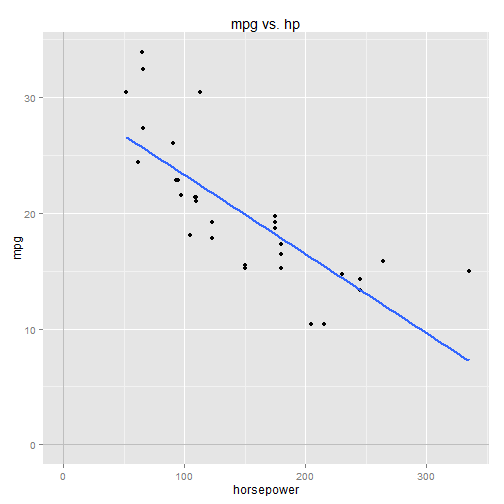

Now we'll include both hp and wt in the same model:
model.hp.wt <- lm(mpg ~ hp + wt, data=mtcars)
summary(model.hp.wt)
## Call:
## lm(formula = mpg ~ hp + wt, data = mtcars)
##
## Residuals:
##    Min     1Q Median     3Q    Max
## -3.941 -1.600 -0.182  1.050  5.854
##
## Coefficients:
##             Estimate Std. Error t value Pr(>|t|)
## (Intercept) 37.22727    1.59879  23.285  < 2e-16 ***
## hp          -0.03177    0.00903  -3.519  0.00145 **
## wt          -3.87783    0.63273  -6.129 1.12e-06 ***
## ---
## Signif. codes:  0 ‘***’ 0.001 ‘**’ 0.01 ‘*’ 0.05 ‘.’ 0.1 ‘ ’ 1
##
## Residual standard error: 2.593 on 29 degrees of freedom
## Multiple R-squared:  0.8268,    Adjusted R-squared:  0.8148
## F-statistic: 69.21 on 2 and 29 DF,  p-value: 9.109e-12
Notice that the coefficients for wt and hp have changed going from the simple models to the multiple regression model.
- mpg is the response variable
- \(\beta_0\) is the Y-intercept
- \(\beta_1\) and \(\beta_2\) are coefficients for the regressor variables
- \(\epsilon\) is the error term (the residuals)
Visualizing the model
One thing to note is that you no longer can visualize the model on a 2D graph, since there are three variables under consideration (the response variable and the two regressors). You need a third axis for the third variable.
So it's possible to graph the model in 3 dimensions, and you could even imagine what it would look like. Imagine a cube, where one corner is the origin of the graph, and the x, y, and z axes go off in each of the three dimensions. The y-axis represents mpg, the x-axis represents hp, and the z-axis represents wt. The regression "line" is actually a 2D plane cutting thru the cube.
- going along the x-axis by hp,
- then rising along the y-axis by \(\beta_1 \cdot hp\),
- then going along the z-axis by wt,
- then rising again along the y-axis by \(\beta_2 \cdot wt \).
Visualizing 4D models...
While it's possible to visualize a regression line with two regressors in 3D space, once you get to three or more regressors it's pretty much impossible to visualize the model, unless you can manage to visualize 4D space (which you can't. Your brain just can't do it).
So we use lower-dimensional models to visualize the models and build intuition about regression in general. Once we get beyond two regressors into higher-dimensional models, we can no longer visualize the model, so we have to apply our intuition abstractly.
Interpreting the multiple regression coefficients
Neither \(\beta_1\) nor \(\beta_2\) are changed by shifting the data. The only thing that changes is the Y-intercept, \(\beta_0\), which can now be interpreted as the predicted mpg for cars with average hp and average wt.
What about the other coefficients? Let's imagine that wt is held constant at wt=mean(wt), so the \(\beta_2\) term drops out: $$ \begin{align*} mpg &= \beta_0 + \beta_1 \cdot (hp - mean(hp)) + \beta_2 \cdot (0) \\[8pt] mpg &= \beta_0 + \beta_1 \cdot (hp - mean(hp)) \end{align*} $$So, like in our single regressor model, \(\beta_1\) is the slope, or the change-in-mpg per change-in-hp. But remember that we're holding wt constant at wt=mean(wt), so what we're actually saying is that \(\beta_1\) is the change-in-mpg per change-in-hp while holding wt constant at wt=mean(wt).
By holding wt constant at wt=mean(wt), we've reduced the equation to just two variables, so we can graph it on a 2D chart as just a straight line with slope \(\beta_1\) and Y-intercept \(\beta_0\).# center the model
model.hp.wt <- lm(mpg ~ I(hp-mean(hp)) + I(wt-mean(wt)), data=mtcars)
summary(model.hp.wt)
## Call:
## lm(formula = mpg ~ I(hp - mean(hp)) + I(wt - mean(wt)), data = mtcars)
##
## Residuals:
## Min 1Q Median 3Q Max
## -3.941 -1.600 -0.182 1.050 5.854
##
## Coefficients:
## Estimate Std. Error t value Pr(>|t|)
## (Intercept) 20.09062 0.45846 43.822 < 2e-16 ***
## I(hp - mean(hp)) -0.03177 0.00903 -3.519 0.00145 **
## I(wt - mean(wt)) -3.87783 0.63273 -6.129 1.12e-06 ***
## ---
## Signif. codes: 0 '***' 0.001 '**' 0.01 '*' 0.05 '.' 0.1 ' ' 1
##
## Residual standard error: 2.593 on 29 degrees of freedom
## Multiple R-squared: 0.8268, Adjusted R-squared: 0.8148
## F-statistic: 69.21 on 2 and 29 DF, p-value: 9.109e-12
B0 <- coef(model.hp.wt)["(Intercept)"]
B1 <- coef(model.hp.wt)["I(hp - mean(hp))"]
B2 <- coef(model.hp.wt)["I(wt - mean(wt))"]
qplot(x=hp-mean(hp), y=mpg, data=mtcars) +
ggtitle("mpg vs. hp, wt=mean(wt)") +
xlab("horsepower") +
geom_abline(intercept = B0 + B2*0, slope = B1) +
geom_vline(x=0, colour="gray") +
geom_hline(y=0, colour="gray")
\(\beta_2 \cdot (2)\) is just another constant term, like \(\beta_0\) so it has no affect on the slope associated with hp, \(\beta_1\). The only thing that has changed is the Y-intercept, which is now \([\beta_0 + \beta_2 \cdot (2)]\).
Again we could graph this on a 2D chart as another straight line, parallel to the line at wt=mean(wt), with a Y-intercept of \(\beta_0 + \beta_2 \cdot 2\).qplot(x=hp-mean(hp), y=mpg, data=mtcars) +
ggtitle("mpg vs. hp, wt=mean(wt) and wt=mean(wt)+2") +
geom_point(mapping=aes(x=hp-mean(hp), y=mpg+B2*2), data=mtcars, colour=6) +
xlab("horsepower") +
ylab("mpg") +
geom_abline(intercept = B0 + B2*0, slope = B1) +
geom_abline(intercept = B0 + B2*2, slope = B1, colour=6) +
geom_vline(x=0, colour="gray") +
geom_hline(y=0, colour="gray")
The pink dots are the same as the block dots, shifted down by the wt factor, \(\beta_2 \cdot 2\).
We could hold wt constant at various levels and end up with a bunch of parallel lines, all with the same slope but different Y-intercepts. If you imagine a z-axis extending into (and out of) the chart, each of those parallel lines exists at a different point along the z-axis, corresponding to the different values for wt. Taken together, the parallel lines form the 2D plane of the regression model.
Similarly, \(\beta_2\) can be interpreted as the change-in-mpg per change-in-wt while holding hp constant. If we hold hp constant at hp=mean(hp), the \(\beta_1\) term drops out: $$ \begin{align*} mpg &= \beta_0 + \beta_1 \cdot (0) + \beta_2 \cdot (wt - mean(wt)) \\[8pt] mpg &= \beta_0 + \beta_2 \cdot (wt - mean(wt)) \end{align*} $$Again, we could hold hp constant at any value and the only thing that would change is the Y-intercept. The slope relating wt to mpg, \(\beta_2\), does not change.
Generally speaking for multiple regression models, the coefficients of the regressor variables can be interpreted as the change-in-response per change-in-regressor while holding all other regressors constant.Calculating the coefficients in a multiple regression model
In order to calculate a regressor's coefficient in a multiple regression model, we must first "regress out" all other regressor variables from both the regressor in question and the response variable. We did this in part 7 for the multiple regression model with hp and am (transmission type) as regressors. Let's do it again here, to build up our understanding and intuition.
By "regress out", we mean to "remove any correlative influence" of one variable from another, so that we can examine the variable in "isolation", so to speak. We do this by building a simple regression model for the two variables, treating one as the response and the other as the regressor (the one being "regressed out"), then taking the residuals and making some use of them (e.g. correlating them with another variable).
The residuals represent the "leftover" variance in the response variable after removing (i.e. "accounting for") any correlative relationship with the regressor variable. In other words, the residuals represent the portion of the response variable's variance that is NOT explained by the regressor variable.
So the logical next step would be to try to correlate this unexplained variance with another regressor's variance, to see how well the other regressor variable can explain this "leftover" variance.
However we can't just directly compare the residuals with another regressor, because this 2nd regressor may be correlated with the first regressor (the one we just "regressed out" of the response). In other words, a portion of the 2nd regressor's variance may already be explained by the first regressor (if they're correlated).
We must remove this correlative influence first, to "isolate" the 2nd regressor from the first regressor, before considering the 2nd regressor's effect on the unexplained/"leftover" variance of the response variable. We do this by building another simple regression model, with the 2nd regressor acting as the response variable and the first regressor acting as the regressor, then taking the residuals. The residuals represent the variance of the 2nd regressor that is NOT explained by the first regressor.
Then we compare the two sets of residuals. We're comparing the unexplained variance of the response variable with the unexplained variance of the 2nd regressor, to determine the correlation between them, after removing ("regressing out") the influence of the first regressor.
I'm not sure I explained that well. Let's work thru the example and hopefully it will become more clear.
In our multiple regression model, we have one response variable (mpg) and two regressors (hp and wt). First up, we want to calculate \(\beta_1\), the coefficient for regressor hp. The coefficient will tell us how mpg "moves" w/r/t hp, while holding all other regressors (wt) constant.
We can't actually hold wt constant in the dataset, simple because in reality the wt variable varies from car to car. By "holding wt constant", what we really mean is, "remove the effect of wt from the model", which we can do by regressing it out of both the response variable (mpg) and the regressor variable (hp). Then we take the residuals from both models and correlate them, which tells us how mpg moves w/r/t hp after the effect of wt has been removed from both.
model.mpg.wt <- lm( mpg ~ wt, data=mtcars )
model.hp.wt <- lm( hp ~ wt, data=mtcars )

model.mpg.wt.resid <- resid(model.mpg.wt)
model.hp.wt.resid <- resid(model.hp.wt)

model.mpg.hp <- lm( model.mpg.wt.resid ~ model.hp.wt.resid )
summary(model.mpg.hp)
## Call:
## lm(formula = model.mpg.wt.resid ~ model.hp.wt.resid)
##
## Residuals:
##    Min     1Q Median     3Q    Max
## -3.941 -1.600 -0.182  1.050  5.854
##
## Coefficients:
##                     Estimate Std. Error t value Pr(>|t|)
## (Intercept)       -3.040e-16  4.507e-01   0.000   1.0000
## model.hp.wt.resid -3.177e-02  8.878e-03  -3.579   0.0012 **
## ---
## Signif. codes:  0 '***' 0.001 '**' 0.01 '*' 0.05 '.' 0.1 ' ' 1
##
## Residual standard error: 2.55 on 30 degrees of freedom
## Multiple R-squared:  0.2992, Adjusted R-squared:  0.2758
## F-statistic: 12.81 on 1 and 30 DF,  p-value: 0.001197

qplot(x=model.hp.wt.resid, y=model.mpg.wt.resid) +
    ggtitle("residuals vs residuals") +
    ylab("residuals of mpg ~ wt") +
    xlab("residuals of hp ~ wt") +
    geom_hline(y=0,colour="lightgray") +
    geom_vline(x=0,colour="lightgray") +
    geom_abline(intercept = coef(model.mpg.hp)[1], slope = coef(model.mpg.hp)[2])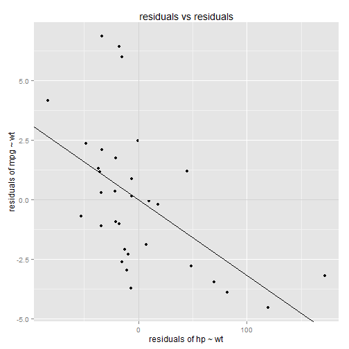
Let's think about this chart for a minute. The y-axis measures the residuals of mpg after wt has been removed. The x-axis measures the residuals of hp after wt has been removed. Variance along the y-axis shows us how mpg "moves" after wt has been accounted for. Variance along the x-axis shows us how hp "moves" after wt has been accounted for. Comparing the two sets of residuals to each other shows us how mpg and hp "move together", after the effect of wt has been removed from both of them.
There's a clear negative correlation in the residuals (I've overlaid the plot with the regression line). This tells us that mpg decreases as hp increases, regardless of vehicle wt. This agrees with our intuitive explanations (higher hp means lower mpg, regardless of wt).
The slope of this regression line gives us the \(\beta_1\) coefficient for the multiple regression model. Note from the model summary that the slope matches up with the \(\beta_1\) coefficient from the multiple regression model.
We do the same procedure to determine the wt coefficient, \(\beta_2\). This time we must regress hp out of both mpg and wt.
model.mpg.hp <- lm( mpg ~ hp, data=mtcars )
model.wt.hp <- lm( wt ~ hp, data=mtcars )

model.mpg.hp.resid <- resid(model.mpg.hp)
model.wt.hp.resid <- resid(model.wt.hp)

model.mpg.wt <- lm( model.mpg.hp.resid ~ model.wt.hp.resid )
summary(model.mpg.wt)
## Call:
## lm(formula = model.mpg.hp.resid ~ model.wt.hp.resid)
##
## Residuals:
##    Min     1Q Median     3Q    Max
## -3.941 -1.600 -0.182  1.050  5.854
##
## Coefficients:
##                     Estimate Std. Error t value Pr(>|t|)
## (Intercept)       -1.154e-16  4.507e-01   0.000        1
## model.wt.hp.resid -3.878e+00  6.221e-01  -6.233 7.27e-07 ***
## ---
## Signif. codes:  0 '***' 0.001 '**' 0.01 '*' 0.05 '.' 0.1 ' ' 1
##
## Residual standard error: 2.55 on 30 degrees of freedom
## Multiple R-squared:  0.5643, Adjusted R-squared:  0.5498
## F-statistic: 38.86 on 1 and 30 DF,  p-value: 7.273e-07

qplot(x=model.wt.hp.resid, y=model.mpg.hp.resid) +
    ggtitle("residuals vs residuals") +
    ylab("residuals of mpg ~ hp") +
    xlab("residuals of wt ~ hp") +
    geom_hline(y=0,colour="lightgray") +
    geom_vline(x=0,colour="lightgray") +
    geom_abline(intercept = coef(model.mpg.wt)[1], slope = coef(model.mpg.wt)[2])