Intro to Statistics: Part 18: Type I Errors, Type II Errors, and Statistical Power

Up to this point, we've been dealing with the analysis of experimental data after the experiment has already been conducted and the data collected. From these analyses we've developed a basic understanding of how things like sample size and effect size influence statistical signficance testing.

We can use this knowledge prior to conducting the experiment to give us an idea of how we should design the experiment, e.g. how big our sample size needs to be, given an anticipated effect size, in order to produce statistically significant results. This is what statisical power is all about.

Type I and Type II errors

Before we delve into statistical power, let's first introduce a few terms we've yet to cover in this series, even though we've been working with the concepts all along. When conducting experiments that study an effect or difference between samples -- e.g. the difference in people's heights, or the effect of a drug on reducing cholesterol -- the following two statements are always true:

There may or may not exist a real effect (or difference) between the groups under study
An effect may or may not be observed in the experimental results, regardless of whether or not a real effect exists

That is to say, there might be a real difference between the heights of Norwegians and everyone else, but that doesn't necessarily mean you will be able to detect it in your sample data. And conversely, you might detect a difference in your sample data, but that doesn't necessarily mean there's a real difference between the full populations.

These two types of experimental errors are known as Type I and Type II errors:

A Type I error is what you would call a "false hit" or a "false positive". It happens when you detect an effect in your sample data, even though no real effect truly exists in the population.
A Type II error is what you would call a "false miss" or "false negative". It happens when you do not detect an effect in your sample data, even though a real effect truly does exist in the population.

The p-value of a significance test gives the probability of a Type I error in your sample data. The p-value is the probability of observing your sample result under the assumption that the null hypothesis (no effect/difference) is true. Even if the null hypothesis is indeed true (there truly is no real effect), it is still possible to observe an effect in your sample data, by random chance due to sampling error. If that happens, that would be a Type I error, and the p-value gives you the probability that such an error has occurred.

The Type I error rate is synonymous with the significance level of the significance test. This is the value chosen (somewhat arbitrarily) by the researcher when deciding whether or not the p-value is small enough to reject the null hypothesis. The significance level is conventionally chosen to be 0.05 and is typically denoted by the greek letter α (alpha), α=0.05. If the p-value is smaller than α, then it's considered significant enough to reject the null hypothesis. Essentially, the Type I error rate (the significance level) is the largest probability of incurring a Type I error that we're willing to accept in our significance test.

The Type II error rate (typically denoted by the greek letter β (beta)) is the rate at which a Type II error might occur. Significance testing doesn't make use of the Type II error rate, however it plays an important role in determining the statistical power of an experiment.

The Type I error rate and Type II error rate are inversely related. The smaller the Type I error rate, the larger the Type II error rate. In other words, the more difficult you make it to observe a statistically significant effect (i.e. the smaller the Type I error rate), the more likely you'll fail to observe an effect that's really there (the Type II error rate).

Statistical power

The statistical power of a significance test is the probability that the test will correctly detect an effect (or difference) in the sample data, assuming a real effect truly exists. In terms of hypotheses, it's the probability of correctly accepting the alternative hypothesis (that an effect exists) and rejecting the null hypothesis (that no effect exists).

In terms of Type I and Type II errors, since we're assuming a real effect exists, then we're not worried about Type I errors, since a "false positive" is impossible given that assumption. We're only concerned with Type II errors, "false negatives", i.e. failing to detect an effect that's really there and, thus, incorrectly accepting the null hypothesis. Statisical power is about minimizing the probability of Type II errors, i.e. minimizing the Type II error rate. Power is defined as the probability of not incurring a Type II error, which is equivalent to (1 - Type II error rate).

The statistical power of an experiment depends on the following factors:

The significance level (Type I error rate, α)
The effect size, which is the magnitude of the difference between the expected outcome (with the effect - the test group) and the null hypothesis (no effect - the baseline or control group)
The sample size

Certain experiments may depend on other factors as well, but these three are the most common.

Power analysis example

To see how these factors affect power, let's work thru an example. Let's revisit the Norwegian heights example from previous articles. In this example we're comparing the average height of Norwegians against the average height of the rest of the world. Let's say the global average height is 67in. We want to conduct an experiment to see if Norwegians are taller, on average.

Let's say we have a hunch that the effect size -- the magnitude of the difference between Norwegian heights and the global average -- is 1.5in. We plan on measuring 30 Norwegians, so our sample size is N=30.

What's the power of this experiment?

If we assume the effect size is 1.5in, then we're assuming the Norwegian population mean is 68.5in, and so we should expect our Norwegian sample mean to be around 68.5in. Of course, it may not be exactly 68.5in, given the randomness involved in selecting a sample. We can use the sampling distribution of the mean to give us an idea of how the sample mean would be distributed.

In order to construct the sampling distribution of the mean, we need to know the population variance. We don't know the population variance, and normally we'd use the sample variance as an estimate. But we haven't conducted the experiment yet, so we don't have a sample. So we need to get this information from elsewhere. Let's say that, for whatever reason, we can estimate the population variance to be around 9in^2 (maybe we know this from other studies).

With this information we can construct two sampling distributions: one for the global population, centered around 67in, and one for the Norwegian population, centered around 68.5in.

N <- 30
pop.mean <- 67
nor.mean <- 68.5
pop.var <- 9
se.mean <- sqrt( pop.var / N )

x <- seq(63.5,71.5,0.01)
ggplot() + 
    stat_function(aes(x=x), 
                  fun=dnorm, 
                  arg=list(mean=pop.mean, sd=se.mean),
                  size=1, 
                  colour="blue") +
    stat_function(aes(x=x), 
                  fun=dnorm, 
                  arg=list(mean=nor.mean, sd=se.mean),
                  size=1, 
                  colour="red") +
    ggtitle("Sampling distribution of the mean\n(sample size N=30)") + 
    geom_hline(y=0, colour="darkgray") +
    geom_vline(x=pop.mean, linetype="dashed", colour="blue", size=1) +
    geom_vline(x=nor.mean, linetype="dashed", colour="red", size=1) +
    ylab("Probability density") + 
    xlab("Sample means")  +
    scale_x_continuous(breaks=64:71, labels=64:71)

The blue line is the sampling distribution centered around the global population mean, 67in. This is the sampling distribution we'll use later on for our significance test, when we test whether the Norwegian sample mean is significantly larger than the global population mean.

The red line is the sampling distribution centered around the assumed Norwegian population mean, 68.5in. Even if our assumption is correct, it's still possible that our randomly selected sample will include some sampling error. The sampling distribution gives us the distribution of sample means that we might observe.

For our significance test, let's say we choose the conventional significance level of α=0.05, and let's say we're only concerned with the difference in one direction, so we'll use the one-tailed test. We can use the qnorm function to find where the significance level falls in the distribution.

alpha <- 0.05
alpha.sample.mean <- qnorm(1-alpha, mean=pop.mean, sd=se.mean)
## 67.9

Let's plot the alpha-level sample mean in the chart.

The orange line is the alpha-level sample mean (67.9in) that corresponds to a significance level of α=0.05. The orange-shaded region is the range of sample means that, if we were to observe a Norwegian sample mean in this range, we'd conclude that the result is significant and thus reject the null hypothesis.

As mentioned before, power is equal to the probability of rejecting the null hypothesis. This is the probability of observing a Norwegian sample mean greater than the alpha-level sample mean, 67.9in. If we assume the Norwegian population mean is 68.5in, we can use the sampling distribution centered around the Norwegian population mean to determine the probability of observing a sample mean greater than 67.9in. This probability is given by the area of the yellow-shaded region in the chart below.

Note that the yellow-shaded region includes the orange-shaded region. It covers the range of statistically significant sample means (along the x-axis) that overlap across the two sampling distributions.

We can use pnorm to get the probability of observing a sample mean in this yellow-shaded range, using the sampling distribution centered around the Norwegian mean.

1 - pnorm(alpha.sample.mean, mean=nor.mean, sd=se.mean)
## 0.86

So, assuming the Norwegian population mean is 68.5in, and assuming the population variance is 9in^2, and given a sample size of N=30, the probability of observing a Norwegian sample mean greater than 67.9in is 0.86. This is the statistical power of the experiment -- i.e. the probability of rejecting the null hypothesis.

The Type II error rate is: 1 - power = 0.14. This is the probability of getting a Norwegian sample mean that's smaller than the alpha-level sample mean. This probability is represented by the red-shaded region in the chart below:

The red-shaded region covers the range of NON-significant sample means that overlap across the two sampling distributions.

The effect of changing the significance level on power

As mentioned above, power depends in part on sample size and significance level. If we change the significance level, that will move the orange line in the charts above, which will change the alpha-level sample mean and therefore change the probability of observing a sample mean above or below the alpha-level.

For example, if we changed the significance level to α=0.10, that would move the orange line to the left and therefore increase power, since it increases the range of statistically significant outcomes in the Norwegian sampling distribution and therefore increases the likelihood of rejecting the null hypothesis.

alpha <- 0.10
alpha.sample.mean <- qnorm(1-alpha, mean=pop.mean, sd=se.mean)
## 67.7

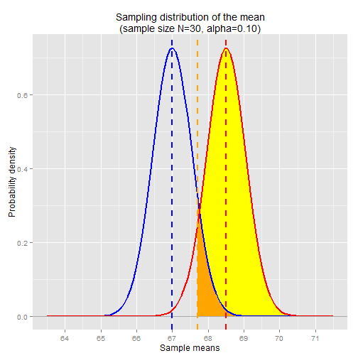
The first chart is the same from above, with α=0.05. The second chart shows the ranges corresponding to α=0.10. The alpha-level sample mean in the second chart dropped to 67.7in, down from 67.9in in the first chart. This increases the range of sample means that are considered statistically significant.

Again we can use pnorm to compute the probability a.k.a power:

1 - pnorm(alpha.sample.mean, mean=nor.mean, sd=se.mean)
## 0.93

Note that by increasing the significance level, we're also increasing the Type I error rate, which means we're increasing the likelihood of incurring a Type I error (false positive). However, as previously mentioned, for a power analysis, we're not concerned with Type I errors, because the power analysis assumes that a real effect exists.

The effect of changing the sample size on power

If we change the sample size, that changes the shape of the sampling distribution. Larger sample sizes result in tighter (narrowly dispersed) sampling distributions, since the variance of the sampling distribution is inversely related to the sample size. This effectively increases power, since it makes it less likely that a Type II error (false negative) will occur.

Smaller sample sizes, on the other hand, result in more widely dispersed sampling distributions, thereby increasing the probability of Type II error and, thus, decreasing the power.

For example, if we reduce the sample size from N=30 to N=10, the chart now looks like this. The significance level is set to α=0.05.

N <- 10
se.mean <- sqrt( pop.var / N )

alpha <- 0.05
alpha.sample.mean <- qnorm(1-alpha, mean=pop.mean, sd=se.mean)
alpha.sample.mean
## 68.6

The alpha-level sample mean jumps to 68.6in, up from 67.9in when the sample size was larger at N=30. Note that the alpha-level sample mean is actually larger than our assumed Norwegian population mean, 68.5in, so in order to get a statistically significant result, we'd have to select a sample that was randomly biased with slightly above-average-heighted Norwegians.

Again we can use pnorm to compute the probability and power:

1 - pnorm(alpha.sample.mean, mean=nor.mean, sd=se.mean)
## 0.47

With a sample size of N=10, power has been reduced to 0.47, down from 0.86 when the sample size was N=30. This means there's only a 47% chance we'll observe a statistically significant difference between the Norwegian sample mean and the global population mean, even when we assume the Norwegian population mean is truly larger than the global population mean.

Recap

A random variable is described by the characteristics of its distribution
The expected value, E[X], of a distribution is the weighted average of all outcomes. It's the center of mass of the distribution.
The variance, Var(X), is the "measure of spread" of a distribution.
The standard deviation of a distribution is the square root of its variance
A probability density function for continuous random variables takes an outcome value as input and returns the probability density for the given outcome
The probability of observing an outcome within a given range can be determined by computing the area under the curve of the probability density function within the given range.
A probability mass function for discrete random variables takes an outcome value as input and returns the actual probability for the given outcome
A sample is a subset of a population. Statistical methods and principles are applied to the sample's distribution in order to make inferences about the true distribution -- i.e. the distribution across the population as a whole
The sample variance is a biased estimate of the true population variance. The bias can be adjusted for by dividing the sum-of-squares by n-1 instead of n, where n is the sample size.
A summary statistic is a value that summarizes sample data, e.g. the mean or the variance
A sampling distribution is the distribution of a summary statistic (e.g. the mean) calculated from multiple samples drawn from an underlying random variable distribution
The Central Limit Theorem states that, regardless of the underlying distribution, the sampling distribution of the mean is normally distributed, with its mean equal to the underlying population mean and its variance equal to the underlying population variance divided by the sample size
An outcome's z-score is calculated by taking the difference between the outcome and the mean, then dividing by the standard deviation. A z-score is in units of standard deviations.
A statistical significance test gives the probability of observing a given outcome under the assumption of a null hypothesis. The probability is known as the p-value for the test. A p-value <= 0.05 is typically considered significant.
A Type I error, a.k.a. a "false positive", is when you incorrectly detect an effect in the sample data even though no real effect exists
A Type II error, a.k.a. a "false negative", is when you incorrectly fail to detect an effect in the sample data even though a real effect truly exists
The significance level, α, for a statistical significance test is the maximum allowed p-value that is considered significant. This is also known as the Type I error rate
The Type II error rate, β, is the probability of incurring a Type II error (false negative)
The t-distribution is used for statistical significance tests when the sample size is small and/or when the true population variance is unknown and therefore estimated from the sample.
The sampling distribution of the variance follows a scaled chi-squared distribution with degrees of freedom equal to n-1, where n is the sample size.
Analysis of variance and F-tests are used for statistical significance testing between three or more samples.