Intro to Statistics: Part 15: The t-distribution

Back in part 12 of this series, we showed how to do a statistical significance test using z-scores.  First we converted the sample mean to a z-score:

Then we plotted the sample mean's z-score against the sampling distribution of the mean, to determine the probability of observing a sample mean as extreme as the one we observed, given the assumptions of the null hypothesis.  Since the sample mean was standardized to a z-score, we used the standard normal distribution as the sampling distribution of the mean for the significance test.

By using the standard normal distribution as the sampling distribution of the mean, we're making the assumption that the z-score for the sample mean is 100% accurate.  However, the z-score calculation depends, in part, on the true population variance, which is typically unknown.  So we use the sample variance as an estimate.  Hence, our z-score, too, is just an estimate. As such it may include some error that we're not accounting for when we use the standard normal distribution.

This is where the t-distribution comes in.  The t-distribution serves (in this context) as a better estimate of the sampling distribution of the mean than the standard normal distribution, especially when the sample size is small, or when the underlying population variance is unknown and therefore has to be estimated from the sample.  

You can read the wikipedia page to find out more about the t-distribution, including its derivation and the theory behind it.  But all you really need to know (for now) is that the t-distribution should be used for significance tests when the sample size is small and/or the underyling population variance is estimated.  The t-distribution attempts to account for the extra bit of error that arises when unknown population statistics, such as variance, are estimated from small samples.

Like the chi-squared distribution, the t-distribution is a family of distribution curves, where each curve in the family is associated with a certain degrees of freedom.  The t-distribution is, in part, derived from the chi-squared distribution (again, check out wikipedia for details). 

Revisiting the statistical significance test example, using the t-distribution

Let's re-do the significance test from part 12, this time using the t-distribution instead of the standard normal distribution.  

Recall that this example involved comparing the difference in heights between our Norwegian sample and the global average.  For the null hypothesis we assumed that the true Norwegian population mean is no different than the global average height.  Given this assumption, we determined the probability of observing the Norwegian sample mean by plotting it in the sampling distribution of the mean, which we constructed using the assumed population mean (from the null hypothesis) and the estimated population variance (from the sample).  This gave us the p-value for our significance test.  

The p-value was quite small, p=0.003, meaning there's only a 0.3% chance of observing such a skewed sample mean, given the null-hypothesis assumption that the Norwegian population mean is truly the same as the global average height.  Since the probability is so minute, we rejected the null-hypothesis assumption, in favor of the alternate hypothesis, which is that the Norwegian population mean is in fact taller than the global average.

First thing we did for the significance test was convert the Norwegian sample mean to a z-statistic (a.k.a. z-score). For t-distributions, we convert to a t-statistic (or t-score) instead. The t-statistic is basically calculated the same way as the z-statistic.  The only difference is that the z-statistic is based on the underlying population variance (which is unknown in this example), whereas the t-statistic is based on the unbiased sample variance.

Recall the sample variance for this example is 9in^2.  Let's assume this is the biased sample variance.  We showed in part 13 that the sample variance is biased by a factor of (n - 1) / n.   The unbiased sample variance is calculated by multiplying the biased variance by the inverse of the bias factor:

The true Norwegian population mean we assume to be 67in (the null hypothesis), and the Norwegian sample mean we said is 68.5in.  The t-statistic is therefore:

Now let's plot our t-statistic in the t-distribution to see where it lands.  As mentioned above, the t-distribution is not a single distribution curve but rather a family of distribution curves, with each curve corresponding to a particular degrees of freedom.  The degrees of freedom for our t-statistic is n - 1, the same as the degrees of freedom for the unbiased sample variance which we  used in the calculation of the t-statistic.  So we plot our t-statistic against the t-distribution curve with degrees of freedom equal to n - 1.

N <- 30
s <- 3.1
nor.mean <- 68.5
pop.mean <- 67
nor.tscore <- (nor.mean - pop.mean) / (s / sqrt(N))

x <- seq(-4.5,4.5,0.01)
shade_x <- seq(nor.tscore,4.5,0.01)
shade_y <- dnorm(shade_x)
shade <- data.frame( rbind(c(nor.tscore,0), cbind(shade_x,shade_y), c(4.5,0)) )

ggplot() + 
    stat_function(aes(x=x), 
                  fun=dt, 
                  args=list(df=N-1),
                  size=1, 
                  colour="blue") +
    ggtitle("t-distribution, degrees of freedom = N-1 = 29") + 
    geom_hline(y=0, colour="darkgray") +
    geom_vline(x=0, linetype="dashed", colour="red", size=1) +
    geom_vline(x=nor.tscore, linetype="dashed", colour="orange", size=1) +
    geom_polygon(data = shade, aes(shade_x, shade_y), fill="yellow") +
    ylab("Probability density") + 
    xlab("Sample mean t-scores")  +
    scale_x_continuous(breaks=-4:4, labels=-4:4)

Like the R functions dnorm, pnorm, qnorm, and rnorm that deal with normal distributions, we can use the dt, pt, qt, and rt functions when dealing with t-distributions.  Each of these functions takes an additional required parameter, df, for the degrees of freedom, which specifies which t-distribution curve (from the t-distribution family) we're working with.

The p-value for our significance test (the area of the yellow-shaded region above) can be determined using the pt function with df = N - 1:

1 - pt( 2.650, df=N-1 )
## [1] 0.006

Compare this to the p-value we got using the z-score and the standard normal distribution, p = 0.003.  The p-value from the t-score and t-distribution is twice as large.  This is because the t-distribution has "fatter tails" than the standard normal.  "Fatter tails" correspond to higher probabilities for extreme outcomes which fall far from the mean (out in the "tails" of the distribution).

In the context of our significance test, the t-distribution represents the sampling distribution of the mean.  So it's basically giving a higher probability of observing sample means that fall far from the population mean, to account for that extra bit of error that gets introduced when we have to estimate the underlying population variance from a small sample.

The t-distribution family

The figure below charts several members of the t-distribution family, each curve with a different degrees of freedom (v).

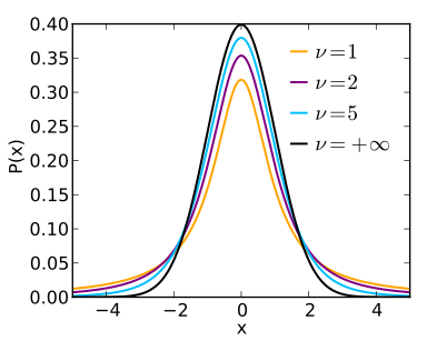
source: wikipedia

The smaller the degrees of freedom, the fatter the tails of the corresponding t-distribution curve (e.g. the orange curve).  The degrees of freedom is related to the sample size, so smaller sample sizes correspond to fatter tails, since small samples have a greater probability of producing sample means that fall far from the true population mean (out in the tails of the distribution).  

As the degrees of freedom increases (which is to say, as the sample size increases), the t-distribution approaches the standard normal distribution (the black curve).  This makes sense, because as the sample size increases, it approaches the population size; therefore the sample estimates become closer approximations of the true population statistics.

Recap

1. A random variable is described by the characteristics of its distribution
2. The expected value, E[X], of a distribution is the weighted average of all outcomes.  It's the center of mass of the distribution.
3. The variance, Var(X), is the "measure of spread" of a distribution.
4. The standard deviation of a distribution is the square root of its variance
5. A probability density function for continuous random variables takes an outcome value as input and returns the probability density for the given outcome
6. The probability of observing an outcome within a given range can be determined by computing the area under the curve of the probability density function within the given range.
7. A probability mass function for discrete random variables takes an outcome value as input and returns the actual probability for the given outcome
8. A sample is a subset of a population. Statistical methods and principles are applied to the sample's distribution in order to make inferences about the true distribution -- i.e. the distribution across the population as a whole
9. The sample variance is a biased estimate of the true population variance.  The bias can be adjusted for by dividing the sum of squared diffs by n-1 instead of n, where n is the sample size.
10. A summary statistic is a value that summarizes sample data, e.g. the mean or the variance
11. A sampling distribution is the distribution of a summary statistic (e.g. the mean) calculated from multiple samples drawn from an underlying random variable distribution
12. The Central Limit Theorem states that, regardless of the underlying distribution, the sampling distribution of the mean is normally distributed, with its mean equal to the underlying population mean and its variance equal to the underlying population variance divided by the sample size
13. An outcome's z-score is calculated by taking the difference between the outcome and the mean, then dividing by the standard deviation.  A z-score is in units of standard deviations.
14. A statistical significance test gives the probability of observing a given outcome under the assumption of a null hypothesis.  The probability is known as the p-value for the test.  A p-value <= 0.05 is typically considered significant.
15. The t-distribution is used for statistical significance tests when the sample size is small and/or when the true population variance is unknown and therefore estimated from the sample.
16. The sampling distribution of the variance follows a scaled chi-squared distribution with degrees of freedom equal to n-1, where n is the sample size.

Intro to Statistics ... 13 . 14 . 15 . 16 . 17 ...