Intro to Statistics: Part 13: Estimating Population Variance from Sample Variance

Typically when you're conducting an experiment to study a particular random variable of nature -- e.g. the heights of random people -- the true values for the mean and variance of the population are not known. They could be determined by rigorously measuring the random variable's value for every member of the population, but this might be experimentally impossible for large population sizes.

So instead, the experimenter takes a randomly selected sample of members from the population, and measures the random variable's value for just the sampled subjects. This gives you a sample, from which you can calculate the sample mean and sample variance. We can then use the sample mean and sample variance as estimates for the true population mean and true population variance.

Sample variance is known as a consistent estimator, which basically means that as the sample size gets larger, the estimate gets closer to the true population variance. This makes sense, since a larger and larger sample size eventually will approach the actual population size, at which point you're calculating the true variance across the entire population.

It turns out, however, that for small sample sizes, the sample variance gives a biased estimate, in that it tends to underestimate the true value of the population variance. This is especially true when the true population mean is also estimated from the sample using the sample mean.

Plotting the sampling distribution of the variance

To help visualize the sample variance bias, let's run a simulation in R where we take a bunch of random samples from the standard normal distribution, with a relatively small sample size of n=20. We'll compute the mean and variance for each sample, then plot the sample variances using a density histogram.

In effect, we're plotting the sampling distribution of the variance (analogous to the sampling distribution of the mean).

set.seed(33)
n <- 20
sample.vars <- NULL

for (i in 1:10000) {
    samp <- rnorm(n)
    sample.mean <- mean(samp)
    sample.var <- sum( (samp-sample.mean)^2 ) / n
    sample.vars <- c(sample.vars, sample.var)
}

ggplot() + 
    geom_histogram(aes(y=..density..,x=sample.vars), 
                   binwidth=0.05, fill="yellow", colour="black") +
    ggtitle("Sampling distribution of the variance") +
    ylab("Probability densities") + 
    xlab("Sample variances (bin width = 0.05) ") +
    geom_vline(x=1,linetype="dashed",size=1.5,colour="blue") +
    geom_vline(x=mean(sample.vars),
               linetype="dashed",size=1.5,colour="orange") 

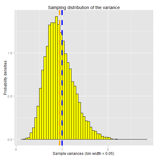
The vertical blue line indicates the true population variance for the standard normal distribution (var=1). The vertical orange line is the mean of the sampling distribution of the variance. As you can see, it slightly underestimates the true population variance.

Adjusting for sample variance bias

Recall that the sample mean and sample variance are calculated by:

\begin{align*}\overline{X} & = \frac{1}{n} \sum_{i=1}^n X_i\\[8pt]\sigma_x^2 & = \frac{1}{n} \sum_{i=1}^n (X_i- \overline{X})^2 \\ \\where, &\\[8pt]n & =  the \ sample \ size\\[8pt]X_1&,\ X_2,\ ...\  X_n \ are \ th…

It can be shown algebraically that the mean of the sampling distribution of the variance underestimates the true population variance by a factor of (n - 1) / n. (Wikipedia works out the derivation, in case you're interested).

\begin{align*}\operatorname{E}[\sigma_x^2] & = \frac{n-1}{n} \cdot \sigma^2\\ \\where, &\\[8pt]\sigma_x^2& = the \ sample \ variance\\[8pt]\sigma^2& = the \ true \ population \ variance\end{align*}

Note that as n becomes very large, (n - 1) / n approaches 1. So as n approaches infinity, the sample variance approaches the true population variance (it is a consistent estimator, as mentioned earlier).

We can correct for this bias by simply multiplying the sample variance by the inverse of the bias factor:

\begin{align*}s^2 & = \frac{n}{n-1} \cdot \sigma_x^2\\[8pt]    & = \frac{n}{n-1} \cdot  \frac{1}{n} \sum_{i=1}^n (X_i- \overline{X})^2 \\[8pt]    & = \frac{1}{n-1} \sum_{i=1}^n (X_i- \overline{X})^2 \\ …

Plotting the unbiased sampling distribution of the variance

Let's re-run the same simulation as before; however this time we'll plot the unbiased sample variances. All the code above stays the same except for the line where we compute the sample variance:

sample.var.unbiased <- sum( (samp-sample.mean)^2 ) / (n-1)

Below is the density histogram of the distribution of unbiased sample variances.

Again, the vertical blue line (hidden behind the orange line) indicates the true population variance (var=1), and the orange line is the mean of the sampling distribution of the (unbiased) variance. The orange line is almost directly on top of the blue line. It's a much closer estimate of the true population variance than the biased estimate above.

So, technically speaking, in the examples we've done in previous articles, where we've estimated the true population variance from the sample variance, we've been (incorrectly) using the biased sample variance. We should have been using the unbiased sample variance.

Note that the effect of the bias gets bigger as the sample size gets smaller. So for small samples (n < 30), it's important to use the unbiased sample variance. For larger n, the bias is small and can often be ignored. When in doubt, just go with the unbiased estimate.

One final note, on the shape of the distribution. Unlike the distribution of sample means, the distribution of sample variances is lower-bounded at 0, because variance can never be a negative number. This causes the distribution to be not quite normally distributed. Instead it follows a chi-squared distribution, which we'll introduce in the next article.

Recap

A random variable is described by the characteristics of its distribution
The expected value, E[X], of a distribution is the weighted average of all outcomes. It's the center of mass of the distribution.
The variance, Var(X), is the "measure of spread" of a distribution.
The standard deviation of a distribution is the square root of its variance
A probability density function for continuous random variables takes an outcome value as input and returns the probability density for the given outcome
The probability of observing an outcome within a given range can be determined by computing the area under the curve of the probability density function within the given range.
A probability mass function for discrete random variables takes an outcome value as input and returns the actual probability for the given outcome
A sample is a subset of a population. Statistical methods and principles are applied to the sample's distribution in order to make inferences about the true distribution -- i.e. the distribution across the population as a whole
The sample variance is a biased estimate of the true population variance. The bias can be adjusted for by dividing the sum of squared diffs by n-1 instead of n, where n is the sample size.
A summary statistic is a value that summarizes sample data, e.g. the mean or the variance
A sampling distribution is the distribution of a summary statistic (e.g. the mean) calculated from multiple samples drawn from an underlying random variable distribution
The Central Limit Theorem states that, regardless of the underlying distribution, the sampling distribution of the mean is normally distributed, with mean equal to the underlying population mean and variance equal to the underlying population variance divided by the sample size
An outcome's z-score is calculated by taking the difference between the outcome and the mean, then dividing by the standard deviation. A z-score is in units of standard deviations.
A statistical significance test gives the probability of observing a given outcome under the assumption of a null hypothesis. The probability is known as the p-value for the test. A p-value <= 0.05 is typically considered significant.

Plotting the sampling distribution of the variance

Adjusting for sample variance bias

Plotting the unbiased sampling distribution of the variance

Recap

Intro to Statistics ... 11 . 12 . 13 . 14 . 15 ...