Intro to Statistics: Part 14: The Chi-Squared Distribution
In the previous article we explored the sampling distribution of the variance -- i.e. the distribution of sample variances computed from many samples drawn from an underlying distribution. We plotted the sampling distribution of the variance and observed that the distribution is lower-bounded at 0, since variance can never be a negative number. This affects the shape of the distribution. Instead of being normally distributed, like the sampling distribution of the mean, the sampling distribution of the variance follows a (scaled) chi-squared distribution.
A chi-squared distribution defines the distribution of a chi-squared random variable. A chi-squared random variable is constructed from the sum-of-squares of a set of k independent standard-normal random variables. A standard-normal random variable is simply a random variable that follows a standard normal distribution. Each random variable in the set is independent of the rest, in the sense that its value doesn't depend on the values of the others.
Another way to think of "k independent standard normal random variables" is to think of them as a sample of k outcomes drawn independently from the standard normal distribution. The value of the chi-squared random variable is computed by squaring each outcome in the sample, then adding up the squares. We'll call this the sum-of-squares statistic for the sample.
![\begin{align*}Q & = \sum_{i=1}^k X_i^2 \\[8pt] & = X_1^2 + X_2^2 + \ ... \ + X_k^2\\ \\Q & \sim \chi_k^2\\ \\ where,\\[8pt]X_1&, \ X_2, \ ... \ X_k \ are \ k \ independent \ standard \ normal \ random \ variables\\[8p…](https://images.squarespace-cdn.com/content/v1/5533d6f2e4b03d5a7f760d21/1434002408147-J022AZTLFS59G7SJ0H0J/image-asset.png)
The distribution of a chi-squared random variable can therefore be thought of as the sampling distribution of the sum-of-squares. Analogous to the sampling distribution(s) of the mean and variance, the sampling distribution of the sum-of-squares is the distribution of the sum-of-squares statistic across multiple samples, all with sample size = k, where all samples are drawn from an underlying standard normal distribution.
The chi-squared family of distributions and the degrees of freedom
The chi-squared distribution is not a single distribution curve but rather a set or family of distribution curves. The parameter that distinguishes one curve from another in the family is called the degrees of freedom.
The degrees of freedom is a statistical term that, in general, indicates the number of "moving parts" that go into the calculation of some statistic. For a chi-squared random variable, the number of moving parts is equal to k -- the number of standard normal random variables that constitute the chi-squared random variable. In terms of samples, the degrees of freedom for a chi-squared random variable is equal to the sample size.
So if our chi-squared random variable consists of 20 standard normal random variables (or a sample of 20 outcomes drawn from the standard normal distribution), then the degrees of freedom = 20. The distribution of a chi-squared random variable consisting of 20 standard normals corresponds to the chi-squared distribution curve with degrees of freedom = 20.
Plotting the sampling distribution of the sum-of-squares
Let's run a simulation in R to plot the sampling distribution of the sum-of-squares. We'll take 10,000 samples of size k=20 from the standard normal distribution (using the rnorm function in R). For each sample we'll compute the sum-of-squares statistic, then plot the distribution of all 10,000 sum-of-squares with a density histogram.
set.seed(33)
k <- 20
sample.SSXs <- NULL

for (i in 1:10000) {
    samp <- rnorm(k)
    sample.ssx <- sum( samp^2 )
    sample.SSXs <- c(sample.SSXs, sample.ssx)
}

ggplot() +
    geom_histogram(aes(y=..density..,x=sample.SSXs),
                   binwidth=1, fill="yellow", colour="black") +
    ggtitle("Sampling distribution of the sum-of-squares\nSample size k=20") +
    ylab("Probability densities") +
    xlab("Sample sum-of-squares (bin width = 1) ") +
    geom_vline(x=k,size=1,colour="blue") +
    geom_vline(x=mean(sample.SSXs),
               linetype="dashed",size=1.5,colour="orange") +
    stat_function(aes(x=sample.SSXs), fun=dchisq, args=list( df=k ),
                  size=0.75, colour="red" )

There's quite a bit going on in this chart so let's break it down. The yellow bars are the density histogram for the sampling distribution of the sum-of-squares. The vertical blue line is the expected value of the chi-squared distribution with degrees of freedom equal to k=20. I haven't mentioned this yet, but the expected value of the chi-squared distribution is equal to its degrees of freedom, so in this example the expected value is 20. The vertical orange line is the actual mean of the sampling distribution of the sum-of-squares. Note that the orange line and the blue line are right on top of each other, which is expected. It means the simulated sampling distribution is consistent with what is theoretically expected from a chi-squared distribution.
The red line is the chi-squared distribution curve with degrees of freedom = 20. It fits the simulated sampling distribution very well.
The effect of the degrees of freedom
Let's re-run the simulation, this time with a sample size/degrees of freedom equal to k=10. All the code from above remains the same except for the setting of k.
k <- 10

The distribution looks similar, only this time everything's centered around 10, which is the degrees of freedom (and expected value) for this chi-squared distribution curve.
The chi-squared distribution family
The following chart shows several members of the chi-squared distribution family. Each curve corresponds to a different degrees of freedom.
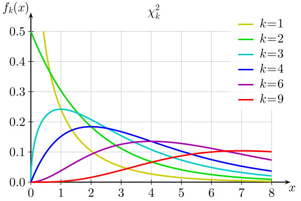
source: Wikipedia
Here you can see the lower-bounded-ness at 0 come into play. When you have only 1 degree of freedom (k=1, the yellow-ish line), that means the chi-squared random variable consists of only 1 standard normal random variable. In terms of samples, it means you're drawing only 1 outcome from the standard normal distribution. Since the standard normal is centered around 0, there's a high probability that you'll draw an outcome close to 0. Recall from the article on standard normals, there's a 68% chance of drawing an outcome between -1 and +1. Squaring that outcome pushes it even closer to 0 (squaring a fraction gives you a smaller fraction). So it makes sense that a chi-squared distribution with degrees of freedom = 1 will have most of its density close to 0, as is shown in the chart. As k increases, the distribution gets pushed out toward higher numbers (the cumulative effect of adding more and more squared values to the chi-squared random variable). As k gets very large, the chi-squared distribution begins to approximate a normal distribution, with the center / mean / expected value at k. (You can't really see that in the chart, because the k values are too small. The simulation above with k=20 illustrates it a little more clearly).
The expected value of the chi-squared distribution is equal to its degrees of freedom.
![\begin{align*}\operatorname{E}[\chi_k^2] & = k\\ \\ where,\\[8pt]k & = degrees \ of \ freedom\end{align*}](https://images.squarespace-cdn.com/content/v1/5533d6f2e4b03d5a7f760d21/1434003885467-CO8AS9T2KLOEXZSE2559/image-asset.png)
How the chi-squared distribution relates to sample variance
The sampling distribution of the variance, which we explored in the previous article, follows a scaled chi-squared distribution:

The scaling factor is:

The population variance for the standard normal distribution is 1, so the scaling factor is simply (n - 1). If you multiply all sample variances by a factor of (n - 1), the resulting distribution follows a chi-squared distribution with n - 1 degrees of freedom.
Let's prove this to ourselves by running another simulation, same as those above, except this time we'll multiple the sample variances by (n - 1) and plot the resulting distribution
set.seed(33)
n <- 10
sample.vars.scaled <- NULL

for (i in 1:10000) {
    samp <- rnorm(n)
    sample.var <- sum( (samp - mean(samp)) ^2 ) / (n-1)
    sample.var.scaled <- sample.var * (n-1)
    sample.vars.scaled <- c(sample.vars.scaled, sample.var.scaled)
}

k <- n-1    # degrees of freedom

ggplot() +
    geom_histogram(aes(y=..density..,x=sample.vars.scaled),
                   binwidth=1, fill="yellow", colour="black") +
    ggtitle(paste("Sampling distribution of the scaled",
                  "sample variance\nSample size n=10")) +
    ylab("Probability densities") +
    xlab("Scaled sample variances (bin width = 1) ") +
    geom_vline(x=k,size=1,colour="blue") +
    geom_vline(x=mean(sample.vars.scaled),
               linetype="dashed",size=1.5,colour="orange") +
    stat_function(aes(x=sample.vars.scaled), fun=dchisq, args=list( df=k ),
size=0.75, colour="red" ) 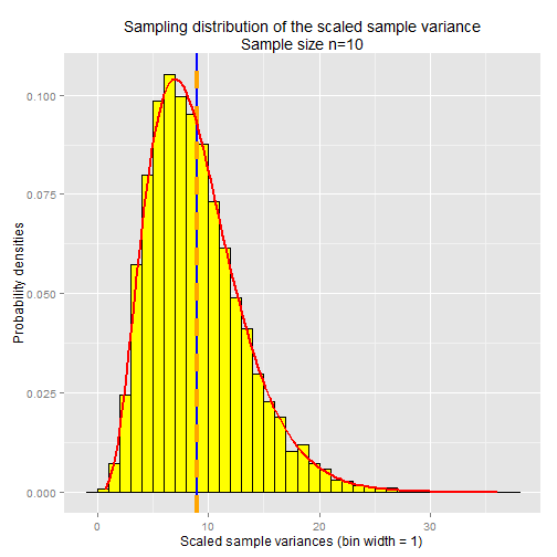
The red line is the chi-squared distribution curve with degrees of freedom k = n - 1. As you can see, it's a close fit to the sampling distribution of the scaled sample variance.
Note that when we multiply the sample variance by the scaling factor, we're left with the sum-of-squared-diffs, i.e. the numerator of the sample variance formula:
 \cdot s^2 &= \sum_{i=1}^n (X_i - \overline{X})^2\end{align*}](https://images.squarespace-cdn.com/content/v1/5533d6f2e4b03d5a7f760d21/1434205632208-K88I6J3941HCZR4HJAC4/image-asset.png)
If we assume that the expected value of the sample mean is 0 (the known population mean for the standard normal distribution), the equation reduces to the sum-of-squares:
![\begin{align*}\operatorname{E}[\overline{X}] &= \mu = 0\\[8pt](n-1) \cdot s^2 &= \sum_{i=1}^n (X_i - 0)^2\\[8pt](n-1) \cdot s^2 &= \sum_{i=1}^n X_i^2\end{align*}](https://images.squarespace-cdn.com/content/v1/5533d6f2e4b03d5a7f760d21/1434205798548-73XQREB7KFZR6T0N6TFL/image-asset.png)
Note that this is the same formula for the chi-squared random variable with degrees of freedom k = n:

You're probably wondering why the sampling distribution of the sample variance doesn't follow a chi-squared distribution with degrees of freedom equal to n, instead of (n - 1). Good question. Well, recall that the sample variance is an estimate of the true population variance. When dealing with estimates, the degrees of freedom is equal to the number of "moving parts" in the system (i.e. the n outcomes in the sample) minus the number of intermediate parameters that go into the calculation of the estimate. The calculation of sample variance uses the sample mean as an intermediate parameter, so we must subtract 1 to account for it. Hence, the degrees of freedom for the sample variance is n - 1.
Another way to think of it is to start off by assuming that the value of the sample variance is known and fixed; therefore it itself is not allowed to move freely within the system. There are n terms that go into the calculation of the sample variance. If we know the first n - 1 of those terms, and we know the resulting value of the calculation (because it is fixed), then we can deduce the value of the nth term using basic algebra. So the nth term technically isn't allowed to move freely in the system either -- its value is dependent on the n - 1 terms before it along with the fixed value for the sample variance. Hence, there are only n - 1 freely moving parts in the system.
Recap
- A random variable is described by the characteristics of its distribution
- The expected value, E[X], of a distribution is the weighted average of all outcomes. It's the center of mass of the distribution.
- The variance, Var(X), is the "measure of spread" of a distribution.
- The standard deviation of a distribution is the square root of its variance
- A probability density function for continuous random variables takes an outcome value as input and returns the probability density for the given outcome
- The probability of observing an outcome within a given range can be determined by computing the area under the curve of the probability density function within the given range.
- A probability mass function for discrete random variables takes an outcome value as input and returns the actual probability for the given outcome
- A sample is a subset of a population. Statistical methods and principles are applied to the sample's distribution in order to make inferences about the true distribution -- i.e. the distribution across the population as a whole
- The sample variance is a biased estimate of the true population variance. The bias can be adjusted for by dividing the sum of squared diffs by n-1 instead of n, where n is the sample size.
- A summary statistic is a value that summarizes sample data, e.g. the mean or the variance
- A sampling distribution is the distribution of a summary statistic (e.g. the mean) calculated from multiple samples drawn from an underlying random variable distribution
- The Central Limit Theorem states that, regardless of the underlying distribution, the sampling distribution of the mean is normally distributed, with its mean equal to the underlying population mean and its variance equal to the underlying population variance divided by the sample size
- An outcome's z-score is calculated by taking the difference between the outcome and the mean, then dividing by the standard deviation. A z-score is in units of standard deviations.
- A statistical significance test gives the probability of observing a given outcome under the assumption of a null hypothesis. The probability is known as the p-value for the test. A p-value <= 0.05 is typically considered significant.
- The sampling distribution of the variance follows a scaled chi-squared distribution with degrees of freedom equal to n-1, where n is the sample size.