Intro to Statistics: Part 12: Statistical Significance Testing Using Z-Scores

In the previous article we introduced the topic of statistical significance testing. The example we used compared the mean height of a sample of Norwegians against the global average height and tested whether the difference between the two means was statistically significant. In this article we'll use the same example, except this time we'll convert everything to z-scores before conducting the significance test. Why? Well, partly because researchers often standardize their results (where "standardize" basically means "convert to z-scores"). But mainly because this exercise will serve as a warm up for later when we introduce t-testing and t-distributions.

Recall that a z-score is calculated by:

We want to standardize the sampling distribution of the mean. Recall the we used the sampling distribution as a way to compare the sample result to the assumptions we made under the null hypothesis -- namely, that the true Norwegian population mean is the same as the global average height: 67in. We estimated the true Norwegian population variance from the sample variance, which we said is 9in^2. That gave us enough information to estimate the sampling distribution of the mean.

\begin{align*}\overline{X} & \sim \operatorname{N}\left(\mu, \frac{\sigma^2}{N}\right )\\[8pt]\operatorname{E}[\overline{X}] & = \mu = 67in\\[8pt]\operatorname{Var}(\overline{X}) & = \frac{\sigma^2}{N} = \frac{3^2}{30}\\[8pt]\operatornam…

So let's standardize the sampling distribution. That's easy: the sampling distribution is a normal distribution, so when we standardize it, it becomes the standard normal distribution, with mean=0 and standard-deviation=1.

Now let's standardize (i.e. convert to a z-score) the Norwegian sample mean, to see where it falls in the standardized sampling distribution:

\begin{align*}Z & = \frac{\overline{X} - \mu}{\frac{\sigma}{\sqrt{N}}}\\[8pt]Z & = \frac{68.5 - 67}{\frac{3}{\sqrt{30}}}\\[8pt]  & = 2.739\end{align*}

In the chart below I've plotted the standard normal distribution. The vertical orange line shows where the Norwegian sample mean z-score falls in the distribution.

N <- 30
sd <- 3
nor.mean <- 68.5
pop.mean <- 67
nor.zscore <- (nor.mean - pop.mean) / (sd / sqrt(N))

x <- seq(-4.5,4.5,0.01)
shade_x <- seq(nor.zscore,4.5,0.01)
shade_y <- dnorm(shade_x)
shade <- data.frame( rbind(c(nor.zscore,0), cbind(shade_x,shade_y), c(4.5,0)) )

ggplot() + 
    stat_function(aes(x=x), 
                  fun=dnorm, 
                  size=1, 
                  colour="blue") +
    ggtitle("Standardized sampling distribution\n(sample size N=30)") + 
    geom_hline(y=0, colour="darkgray") +
    geom_vline(x=0, linetype="dashed", colour="red", size=1) +
    geom_vline(x=nor.zscore, linetype="dashed", colour="orange", size=1) +
    geom_polygon(data = shade, aes(shade_x, shade_y), fill="yellow") +
    ylab("Probability density") + 
    xlab("Sample mean z-scores")  +
    scale_x_continuous(breaks=-4:4, labels=-4:4)

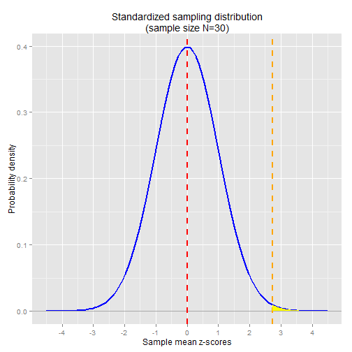
The area shaded in yellow is the probability of observing a sample mean z-score as extreme as the Norwegian sample mean. As in the previous article, we can calculate the probability in R using the pnorm function:

1 - pnorm(2.739)
## [1] 0.003

Note that this is the exact same p-value we got in the non-standardized significance test.

Recap

A random variable is described by the characteristics of its distribution
The expected value, E[X], of a distribution is the weighted average of all outcomes. It's the center of mass of the distribution.
The variance, Var(X), is the "measure of spread" of a distribution.
The standard deviation of a distribution is the square root of its variance
A probability density function for continuous random variables takes an outcome value as input and returns the probability density for the given outcome
The probability of observing an outcome within a given range can be determined by computing the area under the curve of the probability density function within the given range.
A probability mass function for discrete random variables takes an outcome value as input and returns the actual probability for the given outcome
A sample is a subset of a population. Statistical methods and principles are applied to the sample's distribution in order to make inferences about the true distribution -- i.e. the distribution across the population as a whole
A summary statistic is a value that summarizes sample data, e.g. the mean or the variance
A sampling distribution is the distribution of a summary statistic (e.g. the mean) calculated from multiple samples drawn from an underlying random variable distribution
The Central Limit Theorem states that, regardless of the underlying distribution, the sampling distribution of the mean is normally distributed, with mean equal to the underlying population mean and variance equal to the underlying population variance divided by the sample size
An outcome's z-score is calculated by taking the difference between the outcome and the mean, then dividing by the standard deviation. A z-score is in units of standard deviations.
A statistical significance test gives the probability of observing a given outcome under the assumption of a null hypothesis. The probability is known as the p-value for the test. A p-value <= 0.05 is typically considered significant.

Recap

Intro to Statistics ... 10 . 11 . 12 . 13 . 14 ...