Intro to Regression: Part 6: Regressing against a factor variable
Factor variables (aka "nominal" variables) are not numeric, so they require special handling. Let's walk thru an example.
Going back to the mtcars dataset, let's regress mpg against transmission type (am). There are two transmission types: "automatic" and "manual", which are encoded as "0" and "1" in the dataset, respectively.
Just so it's explicitly clear that we're NOT dealing with a numeric variable, I'm going to rename the levels "automatic" and "manual".
data(mtcars)

# convert am to factor and rename levels
mtcars$am <- as.factor(mtcars$am)
levels(mtcars$am) <- c("automatic", "manual")
As per usual, let's first do a scatterplot of mpg vs. transmission type (am):
library(ggplot2)
library(grid)

qplot(x=am, y=mpg, data=mtcars, colour=am) +
    ggtitle("mpg vs. transmission type (am)") +
    xlab("transmission type (am)")
It appears that automatics have lower mpg than manuals, on average.
OK, let's go ahead and build a regression model with mpg as the response variable and transmission type (am) as the sole predictor variable.
model <- lm(mpg ~ am - 1, data=mtcars)This corresponds to the regression model:
- mpg is the response variable
[am == "automatic"]is a "dummy variable"[am == "manual"]is another dummy variable- \(\epsilon\) is the error term (the residuals)
Note: The "-1" in "mpg ~ am - 1" removes the Y-intercept term from the model. Notice that the regression equation above doesn't have a standalone Y-intercept coefficient. Ignore this detail for now, we'll come back to it later.
Dummy variables
Since a factor variable does not have numeric values, we need to
create "dummy variables" for it. That's what [am == "automatic"] and [am == "manual"] represent - they're
both dummy variables.
There's one dummy variable for each factor level. The dummy variable takes on
the value 0 or 1, depending on the value of the factor variable. If the am factor
variable for a particular car equals "automatic", then the [am == "automatic"] dummy
variable is set to 1, while the [am == "manual"] dummy variable is set to 0.
Think of [am == "automatic"] and [am == "manual"] as boolean expressions (note the double "==",
for the programmers out there) that evaluate to true (1) or false (0), depending on the
actual value of the am variable.
Only one dummy variable in the regression function is set to 1 at any given time. The remaining dummy variables are all 0. A dummy variable is set to 1 when the factor variable's value takes on the corresponding factor level.
So in this example we have two factor levels: "automatic" and "manual", and therefore
two dummy variables. When am = "automatic", the [am == "automatic"] dummy variable is 1, while [am == "manual"]
is 0, so it drops out of the equation:
So \(\beta_1\) is the predicted mpg value for "automatic" cars. There is no slope to this equation, it's just a horizontal line at \(Y = \beta_1\), which happens to be the mean(mpg) for cars with am = "automatic".
When am = "manual", the [am == "manual"] variable is set to 1, while the [am == "automatic"] term drops out:
Note that the regression model is not a single line but actually two lines (or points, really), one for each factor level. Let's chart them:
B1 <- coef(model)[1]
B2 <- coef(model)[2]

qplot(x=am, y=mpg, data=mtcars, colour=am) +
    ggtitle("mpg vs. transmission type (am)") +
    xlab("transmission type (am)") +
    geom_hline(y=B1, colour=2) +
    geom_hline(y=B2, colour=5)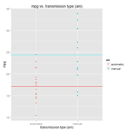
The regression model is two lines:
- the lower line, at predicted mpg = \(\beta_1\) = mean(mpg) for am = "automatic"
- the upper line, at predicted mpg = \(\beta_2\) = mean(mpg) for am = "manual"
If the factor variable had 3 levels, the regression model would have 3 lines. 4 levels, 4 lines. And so on.
Let's look at the model summary to get the coefficient values:
summary(model)
##
## Call:
## lm(formula = mpg ~ am - 1, data = mtcars)
##
## Residuals:
##     Min      1Q  Median      3Q     Max
## -9.3923 -3.0923 -0.2974  3.2439  9.5077
##
## Coefficients:
##             Estimate Std. Error t value Pr(>|t|)
## amautomatic   17.147      1.125   15.25 1.13e-15 ***
## ammanual      24.392      1.360   17.94  < 2e-16 ***
## ---
## Signif. codes:  0 '***' 0.001 '**' 0.01 '*' 0.05 '.' 0.1 ' ' 1
##
## Residual standard error: 4.902 on 30 degrees of freedom
## Multiple R-squared:  0.9487, Adjusted R-squared:  0.9452
## F-statistic: 277.2 on 2 and 30 DF, p-value: < 2.2e-16- \(\beta_1\) = 17.147, the Estimate for the
[am==automatic]coefficient - \(\beta_2\) = 24.392, the Estimate for the
[am==manual]coefficient
Re-introducing the Y-intercept term into the model
Normally you'd include the Y-intercept term in the regression model. For that we need to select a level from the factor variable that represents the "base" level. The Y-intercept coefficient corresponds to the "base" level.
The coefficients for other levels are evaluated relative to the "base" level. This is because the "base" level coefficient (the Y-intercept term) is always present (non-zero) in the regression function.
This is made clear by looking at the regression equation. Without the Y-intercept term, the regression function (from above) is:
The difference being that the [am == "automatic"] dummy variable has been removed.
Thus, [am == "automatic"] represents the "base" level. When the factor variable
equals "automatic", the [am == "manual"] dummy variable drops out, and the
regression equation becomes (ignoring the error term):
So \(\beta_0\) is the predicted mpg when am = "automatic".
When am = "manual", the regression function is: $$ \begin{align*} mpg &= \beta_0 + \beta_1 \cdot [am == "manual"] \\[8pt] mpg &= \beta_0 + \beta_1 \cdot [1] \\[8pt] mpg &= \beta_0 + \beta_1 \end{align*} $$
The predicted mpg when am = "manual" is: \(mpg = \beta_0 + \beta_1\). Contrast this with the non-Y-intercept model above, where
the predicted mpg for am = "manual" is just: \(mpg = \beta_2\). In the Y-intercept model, the Y-intercept coefficient must be
added to the [am == "manual"] coefficient to get the predicted mpg.
This is what I mean when I say the coefficients for other factor levels are evaluated relative to the "base" level. The "base" level coefficient, \(\beta_0\), is always in play. It's never "turned off" for other factor levels.
This affects the coefficients of other levels. When a factor level dummy variable is set to 1, its coefficient is added to \(\beta_0\) to get the predicted mpg. The factor level coefficient represents the difference (in the response variable) between that level and the "base" level.
The linear model including the Y-intercept term
model.y <- lm(mpg ~ am, data=mtcars)
summary(model.y)
##
## Call:
## lm(formula = mpg ~ am, data = mtcars)
##
## Residuals:
##     Min      1Q  Median      3Q     Max
## -9.3923 -3.0923 -0.2974  3.2439  9.5077
##
## Coefficients:
##             Estimate Std. Error t value Pr(>|t|)
## (Intercept)   17.147      1.125  15.247 1.13e-15 ***
## ammanual       7.245      1.764   4.106 0.000285 ***
## ---
## Signif. codes:  0 '***' 0.001 '**' 0.01 '*' 0.05 '.' 0.1 ' ' 1
##
## Residual standard error: 4.902 on 30 degrees of freedom
## Multiple R-squared:  0.3598, Adjusted R-squared:  0.3385
## F-statistic: 16.86 on 1 and 30 DF,  p-value: 0.000285
By default, lm will use the "lowest" level in the factor variable to represent the "base" level (in this example, the lowest level is "automatic"). The coefficients for remaining factor levels represent the difference between that level and the base level. The coefficient values are:
- \(\beta_0\) = 17.147, the Estimate for the (Intercept) coefficient
- \(\beta_1\) = 7.245, the Estimate for the
[am == "manual"]coefficient
Note that \(\beta_0\) from the Y-intercept model equals \(\beta_1\) from the non-Y-intercept model,
which makes sense since they both correspond to [am == "automatic"].
Also note that \(\beta_0 + \beta_1\) from the Y-intercept model equals \(\beta_2\) from the non-Y-intercept
model. This makes sense because the combined coefficients from the Y-intercept model give you the
predicted mpg for [am == "manual"], just as \(\beta_2\) does in the non-Y-intercept model.
The regression lines from the Y-intercept model are identical to those from the non-Y-intercept model:
B0 <- coef(model.y)[1]
B1 <- coef(model.y)[2]

qplot(x=am, y=mpg, data=mtcars, colour=am) +
    ggtitle("mpg vs. transmission type (am)") +
    xlab("transmission type (am)") +
    geom_hline(y=B0, colour=2) +
    geom_hline(y=B0+B1, colour=5)
Again, the regression model is two lines:
- the lower line, at predicted mpg = \(\beta_0\) = mean(mpg) for am = "automatic"
- the upper line, at predicted mpg = \(\beta_0 + \beta_1\) = mean(mpg) for am = "manual"
The residuals
Let's take a look at the residuals for the Y-intercept model:
mpg.actual <- mtcars$mpg
mpg.predicted <- predict(model.y)
mpg.residual <- resid(model.y)

data.frame(mpg.actual, mtcars$am, mpg.predicted, mpg.residual)

hist(mpg.residual,
     col="yellow",
     main="Distribution of mpg residuals",
     xlab="mpg residuals")

##                     mpg.actual mtcars.am mpg.predicted mpg.residual
## Mazda RX4                 21.0    manual      24.39231   -3.3923077
## Mazda RX4 Wag             21.0    manual      24.39231   -3.3923077
## Datsun 710                22.8    manual      24.39231   -1.5923077
## Hornet 4 Drive            21.4 automatic      17.14737    4.2526316
## Hornet Sportabout         18.7 automatic      17.14737    1.5526316
## Valiant                   18.1 automatic      17.14737    0.9526316
## ...
The residuals appear to be distributed somewhat normally. This tells us the prediction errors are somewhat balanced around the regression line(s), which is what we want.
The residuals for the Y-intercept model are exactly the same as the residuals for the non-Y-intercept model:
mpg.actual <- mtcars$mpg
mpg.predicted <- predict(model)
mpg.residual <- resid(model)

data.frame(mpg.actual, mtcars$am, mpg.predicted, mpg.residual)

hist(mpg.residual,
     col="yellow",
     main="Distribution of mpg residuals",
     xlab="mpg residuals")

##                     mpg.actual mtcars.am mpg.predicted mpg.residual
## Mazda RX4                 21.0    manual      24.39231   -3.3923077
## Mazda RX4 Wag             21.0    manual      24.39231   -3.3923077
## Datsun 710                22.8    manual      24.39231   -1.5923077
## Hornet 4 Drive            21.4 automatic      17.14737    4.2526316
## Hornet Sportabout         18.7 automatic      17.14737    1.5526316
## Valiant                   18.1 automatic      17.14737    0.9526316
## ...
Goodness of fit - R
2
Finally, let's calculate R 2 :
ss.res <- sum(mpg.residual^2)
ss.tot <- with(mtcars, sum( (mpg - mean(mpg))^2 ) )

R2 <- 1 - ss.res / ss.tot
## 0.3597989
Note this is the same R 2 reported by the Y-intercept model summary (the "Multiple R-squared" field). It's not that great - only 36% of the variance is explained by the model. But that's not much of a surprise since our model is very simplistic.
Note, however, that it is not the same R 2 reported by the non-Y-intercept model above. For an explanation of this apparent inconsistency, check out this thread: http://stats.stackexchange.com/questions/26176/removal-of-statistically-significant-intercept-term-boosts-r2-in-linear-model