Intro to Statistics: Part 8: Sampling Distributions
Sampling distributions are an important concept to understand. There's nothing terribly complex about them, however if you're like me, you may find them difficult at first. The terminology can be confusing -- some terms are "overloaded", in that they refer to subtly different things depending on the context. This makes sampling distributions somewhat tricky to explain, so bear with me.
Maybe the easiest way to explain sampling distributions is by way of an example.
Let's imagine selecting 10 outcomes at random from a random variable's distribution. For example, let's say you roll a single die 10 times and record the results. These 10 outcomes make up a single sample. The sample size is 10.
Now imagine computing a summary statistic on that sample, for example the sample mean. OK, so far so good.
Now imagine taking yet another sample of 10 die rolls, and again computing the mean for that sample. Now we have two samples and two means, one mean from each sample.
Ok, now let's ramp up this line of thought: Imagine taking multiple separate samples, each with sample size = 10, and computing the mean for each sample. We now have multiple sample means, one mean from each sample. This collection of sample means is called a sampling distribution.
Wikipedia's definition of a sampling distribution is:
The sampling distribution of a statistic is the distribution of that statistic, considered as a random variable, when derived from a random sample of size n. It may be considered as the distribution of the statistic for all possible samples from the same population of a given size.
In the die roll example above, the statistic in question is the mean. A sampling distribution is the distribution of a single summary statistic across all samples. We could have used any statistic. For example instead of the mean we could have computed the variance of each sample, and in the end we'd have the sampling distribution of the variance. Most of the time, however, you'll be working with the sampling distribution of the mean.
Note that the summary statistic is, itself, a random variable, since it is derived from random samples taken from an underlying random variable distribution. The distribution for this summary-statistic random variable is the sampling distribution. Like any other random variable, we can use its distribution (the sampling distribution) to compute things like its mean and variance.
It's important to understand the distinction between the sampling distribution and the underlying random variable distribution from which the sampling distribution is derived. A sampling distribution is the distribution of a sample statistic (e.g the sample mean), whose values are calculated from multiple distinct samples selected randomly from the underlying random variable distribution. Each sample contributes one value to the sampling distribution (or one "outcome", in the random variable sense).
So in other words, to construct a sampling distribution, you would...
- Start with a random variable distribution
- Take multiple samples from the random variable distribution
- Calculate a summary statistic for each of those samples (e.g. the mean of each sample)
- The set of values for the summary statistic (one value per sample) is the sampling distribution of that statistic (e.g. the sampling distribution of the mean)
Sampling distribution example
Let's try to visualize this with an example. We'll use R to simulate taking multiple samples from a random variable with a uniform distribution of outcomes between 1 and 6. In a uniform distribution, each outcome has equal probability. So this is equivalent to rolling a six-sided die a bunch of times and taking samples of the outcomes.
We'll use the runif function to generate our random samples. runif generates uniformly distributed random values in whatever range of possible outcomes you tell it. For this example we'll use the range 1 - 6. Our sample size is N=10.
Aside: runif returns random values for a continuous random variable, not a discrete random variable like our six-sided die. To account for this, we'll generate random values between 0 and 6 and round them all up (i.e take their ceiling). This effectively converts runif from a continuous distribution between 0 and 6 to a discrete distribution between 1 and 6.
The code below uses a for-loop to generate and plot eight samples, all with sample size N=10.
set.seed(1)

N <- 10
sample.means <- NULL
par(mfrow=c(2,4))

# Loop eight times to collect eight samples
# and calculate eight sample means.
for (i in 1:8) {

    # converting from continuous to discrete outcomes between 1 and 6.
    sample <- ceiling( runif( N, 0, 6) )
    sample.mean <- mean(sample)

    plot(x=1:N,
         y=sample,
         main=paste("Sample",i),
         ylim=c(0,6),
         xlab="",
         xaxt='n',
         ylab="Outcomes")
    abline(a=sample.mean,b=0,col="red",lty="dashed")

    # Remember the sample means to graph them later
    sample.means <- c(sample.means, sample.mean)
}

The mean for each sample is plotted as a dashed red line along with the sample data. Recall that the theoretical true mean for a six-sided die is:

The sample means shown above are all in the neighborhood of 3.5, with minor discrepencies due to the randomness of sampling.
We then collect the set of sample means compiled from all samples and plot them below. The set of sample means comprises the sampling distribution of the mean.
# Plot the sample.means; i.e. the sampling distribution of the mean
par(mfrow=c(1,1))
plot(x=1:8,
     y=sample.means,
     col="red",
     main="Sampling distribution of the mean",
     ylim=c(0,6),
     xlab="Samples",
     ylab="Sample means")
abline(a=mean(sample.means),b=0,col="blue",lty="dashed")
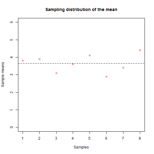
The blue dashed line is the mean of all the sample means. Remember, the mean statistic that we summarized from our samples is a random variable itself, and its distribution is the sampling distribution. The mean of this sampling distribution is the mean of the sample means -- i.e. the mean of the means, or the mean of the sampling distribution of the mean (I warned you about overloaded terminology).
A density histogram of the sampling distribution
Let's run another simulation, again using our six-sided die, but this time let's ramp up the number of samples to 1000 and plot the results using a density histogram.
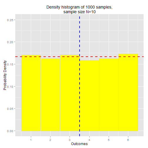

The first chart depicts the density histogram for all sample data. As expected the probability density is uniformly distributed. Since the six-sided die is a discrete random variable, this is technically a probability mass histogram, so the probability density values are the actual probabilities associated with each outcome. Note that the probability for each outcome is approximately 0.1667, or 1/6, which is the true/theoretical probability for each outcome. The red dashed line marks the true probability.
The second chart depicts the density histogram for the sampling distribution of the mean. Notice that the distribution is shaped like a normal distribution, clustered around the mean of the sample means, which is approximately equal to the expected value of the underlying distribution (the six-sided die), E[X] = 3.5. The blue dashed line in both charts indicates the true expected value E[X] = 3.5.
This result should be consistent with our intuitive expectations. The expected value of a random variable is the long-run mean of its outcomes. If we took a random sample of those outcomes and calculated the sample mean, we'd expect the sample mean to be roughly equal to the theoretical expected value of the random variable, more or less. If we took multiple samples and calculated the mean for each, we'd expect those sample means to be clustered around the expected value of the random variable. In other words, we'd expect the sampling distribution of the mean to be clustered around the theoretical expected value of the underlying distribution from which the sample means are derived.
The effect of increasing the sample size
So let's run yet another simulation with our six-sided die, but this time let's increase the sample size to N=30. Again we'll collect 1000 samples.


As you can see, the density histogram for our sample data looks pretty much the same, although now we have more data so the densities of each outcome more closely approximate their true density, 0.16667, or 1/6, as indicated by the red dashed line.
Notice that the sampling distribution in the second chart is even more tightly clustered around the theoretical expected value of the underlying distribution than in the first chart, where we had a smaller sample size. In other words, the variance of the sampling distribution of the mean gets smaller as the sample size gets bigger. This makes sense because with a larger sample size, we'd expect each of our sample means to more closely approximate the true expected value of the random variable.
We're beginning to touch on the Central Limit Theorem, which is one of the most fundamental theories of statistics and serves as the basis for statistical inference. We'll cover the Central Limit Theorem in the next article.
Recap
- A random variable is described by the characteristics of its distribution
- The expected value, E[X], of a distribution is the weighted average of all outcomes, where each outcome is weighted by its probability
- The variance, Var(X), is the "measure of spread" of a distribution. It's calculated by taking the weighted average of the squared differences between each outcome and the expected value.
- The standard deviation of a distribution is the square root of its variance
- A probability density function for continuous random variables takes an outcome value as input and returns the probability density for the given outcome
- The probability of observing an outcome within a given range can be determined by computing the area under the curve of the probability density function within the given range.
- A probability mass function for discrete random variables takes an outcome value as input and returns the actual probability for the given outcome
- A sample is a subset of a population. Statistical methods and principles are applied to the sample's distribution in order to make inferences about the true distribution -- i.e. the distribution across the population as a whole
- A summary statistic is a value that summarizes sample data, e.g. the mean or the variance
- A sampling distribution is the distribution of a summary statistic calculated from multiple samples taken from the underlying random variable distribution