Intro to Statistics: Part 4: Another Example of a Random Variable: Rolling Two Dice
The example random variables we've been using so far, the coin flip and die roll, are similar in that they both have distributions where every outcome has equal probability of occurring. Let's take it up a notch and work thru an example of a random variable whose outcomes have differing probabilities.
Let's consider a random variable X that represents the rolling of, not one, but two dice. The set of outcomes is 2 thru 12, but not every outcome is equally likely. 7s are more likely to occur than 2s or 12s. We can determine the probability of each outcome by examining all possible permutations of tossing two dice.
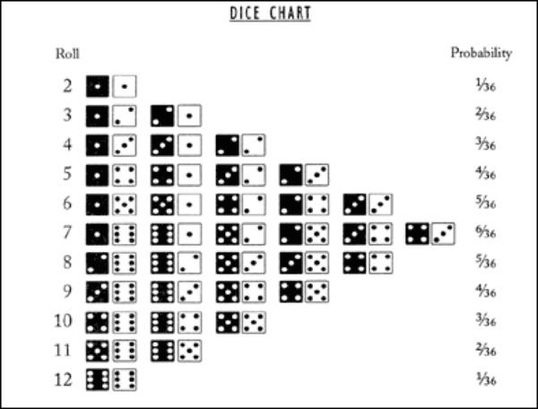
To determine the probability of an outcome, take the number of permutations for that outcome and divide it by the total number of permutations across all outcomes. The "Probability" column in the chart on the right gives the probability for each outcome.
Note that the sum of all probabilities of all outcomes equals 1, as expected.
Expected value
To determine the expected value, simply plug the outcomes and probabilities into the equation:
![\begin{align*}\operatorname{E}[X] = x_1&p_1 + x_2p_2 + \dotsb + x_kp_k \\ \\ = 2 \cdot & \frac{1}{36} + 3 \cdot \frac{2}{36} + 4 \cdot \frac{3}{36} + 5 \cdot \frac{4}{36} + 6 \cdot \frac{5}{36} + 7 \cdot \frac{6}{36}\\ …](https://images.squarespace-cdn.com/content/v1/5533d6f2e4b03d5a7f760d21/1429593820894-20OA53STFR4PR9O8GAM7/image-asset.png)
It makes sense that the expected value is 7, given the perfect symmetry of the permutations shown in the chart above. The expected value can be thought of as the distribution's "center of mass", and it's clear that the permutations balance perfectly at 7.
Variance
We can calculate the random variable's variance by again plugging our values into the equation:
![\begin{align*}\operatorname{Var}(X) = \operatorname{E}&\left[(X - \mu)^2 \right]\\ \\= (&2-7)^2 \cdot \frac{1}{36} + (3-7)^2 \cdot \frac{2}{36} + (4-7)^2 \cdot \frac{3}{36} + (5-7)^2 \cdot \frac{4}{36}\\ \\ & + (6-7)^2 \cdot \frac{5…](https://images.squarespace-cdn.com/content/v1/5533d6f2e4b03d5a7f760d21/1429594715212-8BAMI2AG04GZTT8FUEW9/image-asset.png)
Let's double-check our work using the other form of the variance formula:
![\begin{align*}\operatorname{Var}(X) = \operatorname{E}&[X^2] - \operatorname{E}[X]^2\\ \\ = 2&^2 \cdot \frac{1}{36} + 3^2 \cdot \frac{1}{36} + 4^2 \cdot \frac{1}{36} + 5^2 \cdot \frac{1}{36} + 6^2 \cdot \frac{1}{36} + …](https://images.squarespace-cdn.com/content/v1/5533d6f2e4b03d5a7f760d21/1429595106106-N46CQMFATE03JNFI2YKN/image-asset.png)
Distribution
A common way to chart the distribution of a random variable is with a histogram. A histogram lists the outcomes along the x-axis, while along the y-axis are either the relative frequencies of the outcomes (number of times each outcome occurs relative to other outcomes) or the probability densities of the outcomes.
The chart below plots the relative frequencies of outcomes (we'll cover probability densities in a future post). The relative frequencies are the theoretically expected outcomes if you were to toss two dice 36 times and record the number of times each outcome occurred. According to the theoretical probabilities, out of 36 tosses you should observe a 7 six times, a 6 five times, a 5 four times, and so on.

If you were to plot the expected value on this chart (E[X] = 7), it would be a vertical line that cuts right down the middle of the distribution. As mentioned before, think of the expected value as the balancing point of the distribution, where 50% of the weighted outcomes lie on one side of the line and the other 50% of weighted outcomes lie on the other.
Note that there's no difference in the shape of the distribution whether you plot relative frequencies or probability densities. In fact you can easily convert this chart to a probability density histogram by simply dividing each frequency value on the y-axis by 36. That would convert the theoretical frequencies into the theoretical probabilities, leaving you with a density histogram, but the shape of the histogram would not change.
Craps
For any craps players out there, the dice chart and probabilities shown above illustrate why the "odds bet" (the one you place behind the pass line bet) is valued the way it is. The "odds bet" is one of the only bets in the casino that pays its true odds (there's no house advantage). The payoff on the odds bet depends on the relative likelihood of rolling the point value versus rolling a 7. Rolling the point wins the bet; rolling a 7 loses the bet. If the point is 6, then the odds bet pays off at 6:5 -- which from the chart we can see is the relative probability of rolling a 7 to a 6: 6/36 to 5/36, or simply 6:5. The odds and payouts for the other point values are shown in the chart below:
Point Payoff True odds of rolling a 7 vs the point
4 2:1 6/36 to 3/36 = 6:3 = 2:1
5 3:2 6/36 to 4/36 = 6:4 = 3:2
6 6:5 6/36 to 5/36 = 6:5
8 6:5 6/36 to 5/36 = 6:5
9 3:2 6/36 to 4/36 = 6:4 = 3:2
10 2:1 6/36 to 3/36 = 6:3 = 2:1
Recap
- A random variable is described by the characteristics of its distribution
- Each outcome in the distribution has an associated probability of occurring
- The sum of the probabilities of all possible outcomes equals 1
- The expected value, E[X], of a distribution is the weighted average of all outcomes, where each outcome is weighted by its probability
- The variance, Var(X), is the "measure of spread" of a distribution. It's calculated by taking the weighted average of the squared differences between each outcome and the expected value.
- The standard deviation of a distribution is the square root of its variance
- A random variable's distribution can be plotted using a histogram of either frequencies (counts) or density (probabilities)
- When playing craps, always bet the pass line and always max out your odds bet. It's one of the only "true odds" bets you'll find in the casino